2 Getting Started with R

The aim of this chapter is to get you started with the basic tasks of data analysis using R. A good starting point to learn more about R and a permanent reference is Wickham, Çetinkaya-Rundel, and Grolemund (2023) (available online at this link). There are plenty of other resources, both printed, such as Albert and Rizzo (2012) and Zuur, Ieno, and Meesters (2009), and online including courses at Coursera and CognitiveClass.Ai. Another great resource is Datacamp which allows learning programming in an interactive environment.

The starting point of this chapter is how to load data in R and we will discuss two ways of doing this: loading a data file stored in your computer and downloading the data from the internet. We will introduce R-terminology as needed in the discussion. Once we have loaded data in R it is time to explore the dataset by viewing the data, summarize it with statistical quantities (e.g., the mean), and plotting the variables and their distribution.

The way R works is as follows:

• Object: R stores information (i.e., number or string values) in objects
• Structure: these objects organize information in a different way:
  • data frames are tables with each column representing a variable and each row denoting an observational unit (e.g., a stock, a state, or a month); each column can be of a different type, for example a character string representing an address or a numerical value.
  • matrices are similar to data frames with the important difference that all variables must be of the same type (i.e., all numerical values or characters)
  • lists can be considered an object of objects in the sense that each element of a list could be a data frame or a matrix (or a list)
• Function: is a set of operations that are performed on an object; for example, the function mean() calculates the average of numerical variable by summing all the values and dividing by the number of elements.
• Package: is a set of functions that are used to perform certain tasks (e.g., load data, estimate models etc)

One of the most important functions that you will use in R is help(): by typing the name of a function within the brackets, R pulls detailed information about the function arguments and its expected outcome. With hundred of functions used in a typical R session and each having several arguments, even the most experienced R programmers ask for help().

2.1 Reading a local data file

The file List_SP500.csv is a text file in comma separated values (csv) format that contains information about the 500 companies that are included in the S&P 500 Index¹. The code below shows how to load a text file called List_SP500.csv using the read.csv() function. The output of reading the file is then assigned to the splist object that is stored in the R memory. Anytime we type splist in the command line, R will pull the data contained in the object. For example, the second line of code uses the head(splist, 10) function to print the first 10 rows of the splist object.

splist <- read.csv("List_SP500.csv")
head(splist,10)

   Symbol               Security            GICS.Sector   Headquarters.Location
1     MMM                     3M            Industrials   Saint Paul, Minnesota
2     AOS            A. O. Smith            Industrials    Milwaukee, Wisconsin
3     ABT                 Abbott            Health Care North Chicago, Illinois
4    ABBV                 AbbVie            Health Care North Chicago, Illinois
5     ACN              Accenture Information Technology         Dublin, Ireland
6    ADBE             Adobe Inc. Information Technology    San Jose, California
7     AMD Advanced Micro Devices Information Technology Santa Clara, California
8     AES        AES Corporation              Utilities     Arlington, Virginia
9     AFL                  Aflac             Financials       Columbus, Georgia
10      A   Agilent Technologies            Health Care Santa Clara, California
   Date.added     Founded
1  1957-03-04        1902
2  2017-07-26        1916
3  1957-03-04        1888
4  2012-12-31 2013 (1888)
5  2011-07-06        1989
6  1997-05-05        1982
7  2017-03-20        1969
8  1998-10-02        1981
9  1999-05-28        1955
10 2000-06-05        1999

The object splist represents a data frame in R terminology: a table in which each column represents a variable and each row is a different unit (in this case companies listed in the S&P 500 Index). The splist data frame has 6 columns and 503 rows². The size of the data frame can be found using the dim(splist) command which provides the dimension of the frame, or using ncol(splist) and nrow(splist). The commands head(), dim(), ncol() and nrow() are functions that execute a series of operations on a data objects. The function inputs are referred to as arguments, that, except for the data object, are typically set to default values (in the case of head() the default for argument n is 6). A useful command to obtain the properties of the columns that have been imported is str():

str(splist)

'data.frame':   503 obs. of  6 variables:
 $ Symbol               : chr  "MMM" "AOS" "ABT" "ABBV" ...
 $ Security             : chr  "3M" "A. O. Smith" "Abbott" "AbbVie" ...
 $ GICS.Sector          : chr  "Industrials" "Industrials" "Health Care" "Health Care" ...
 $ Headquarters.Location: chr  "Saint Paul, Minnesota" "Milwaukee, Wisconsin" "North Chicago, Illinois" "North Chicago, Illinois" ...
 $ Date.added           : chr  "1957-03-04" "2017-07-26" "1957-03-04" "2012-12-31" ...
 $ Founded              : chr  "1902" "1916" "1888" "2013 (1888)" ...

The structure of the object provides the following information:

• the object is a data.frame
• number of observations (503) and variables (6)
• name of each variable included in the data frame (Symbol, Security, GICS.Sector, Headquarters.Location, Date.added, Founded)
• type of the variable (chr)

The type refers to the type of data represented by each variable and defines the operations that R can do on the variable. For example, if a numerical variable is mistakenly defined as a string of characters than R will not be able to perform mathematical operations on such variable and produces an error message. The types available in R are:

• numeric: (or double) is used for decimal values
• integer: for integer values
• character: for strings of characters
• Date: for dates
• factor: represents a type of variable (either numeric, integer, or character) that categorizes the values in a small (relative to the sample size) set of categories (or levels)

The structure of the dataset shows that all variables have been imported as character, although this does not seem appropriate for the Date.added variable and the Founded that is a year. We can redefine the type of the variable by setting the variable Date.added in the splist object to be a date as done below:

splist$Date.added <- as.Date(splist$Date.added, format="%Y-%m-%d")
class(splist$Date.added)

[1] "Date"

Notice that:

• $ sign is used to extract a variable/column in a data frame; splist$Date.added extract the Date.added from the data frame object splist
• as.Date() function converts the splist$Date.added from character to Date; the role of the argument format="%Y-%m-%d" is to specify the format of the date being defined³
• class() is a function used to obtain the class type of an object (or the variable in a data frame as in this case).

Although the csv format is probably the most popular for exchanging text files, there are other formats and dedicated functions in R to read these files. For example, read.delim() and read.table() are two functions that can be used for tab-delimited or space-delimited files.

An alternative to using the base function is to employ functions from other packages that presumably improve some aspects of the default function. readr is a package that provides smarter parsing of the variable and save the user some time in redefining variable. Below we apply the function read_csv() from the package readr to import the List_SP500.csv file:

library(readr)
splist <- read_csv("List_SP500.csv")
str(splist, max.level=1)

spc_tbl_ [503 × 6] (S3: spec_tbl_df/tbl_df/tbl/data.frame)
 - attr(*, "spec")=
  .. cols(
  ..   Symbol = col_character(),
  ..   Security = col_character(),
  ..   `GICS Sector` = col_character(),
  ..   `Headquarters Location` = col_character(),
  ..   `Date added` = col_date(format = ""),
  ..   Founded = col_character()
  .. )
 - attr(*, "problems")=<externalptr> 

Some remarks:

• before being able to use functions from a package, it needs to be installed in your local machine. R comes with a few base packages while the more specialized packages have to be installed by the user. This is done with the command install.packages(readr) that needs to be performed only once. After the installation, library(readr) or require(readr) are the commands used to pull the package that make all the functions in the packages available in the R environment. If you call a function from a package that is not loaded, R issues an error message that the function is not known.
• the function read_csv() correctly classifies the variable Date.added as a date.
• the other variables are defined as character instead of factor

The readr package produces an object that is a data frame of class tbl_df. Although the object is still a data frame, the class provides some additional capabilities that will be discussed in more detail in later chapters.

Let’s consider another example. In the previous Chapter we discussed the S&P 500 Index with the data obtained from Yahoo Finance. The dataset was downloaded and saved with name GSPC.csv to a location in the hard drive. We can import the file in R using the read.csv() function:

index <- read.csv("GSPC.csv")
tail(index, 8)

     symbol       date    open    high     low   close     volume adjusted
7300  ^GSPC 2023-12-29 4782.88 4788.43 4751.99 4769.83 3126060000  4769.83
7301  ^GSPC 2024-01-02 4745.20 4754.33 4722.67 4742.83 3743050000  4742.83
7302  ^GSPC 2024-01-03 4725.07 4729.29 4699.71 4704.81 3950760000  4704.81
7303  ^GSPC 2024-01-04 4697.42 4726.78 4687.53 4688.68 3715480000  4688.68
7304  ^GSPC 2024-01-05 4690.57 4721.49 4682.11 4697.24 3844370000  4697.24
7305  ^GSPC 2024-01-08 4703.70 4764.54 4699.82 4763.54 3742320000  4763.54
7306  ^GSPC 2024-01-09 4741.93 4765.47 4730.35 4756.50 3529960000  4756.50
7307  ^GSPC 2024-01-10 4759.94 4790.80 4756.20 4783.45 3498680000  4783.45

where the tail() command is used to print the bottom 8 rows of the data frame. Files downloaded from Yahoo have, in addition to the date, 6 columns that represent the price at the open of the trading day, highest and lowest price of the day, the closing price, the volume transacted, and the adjusted closing price⁴. The structure of the object is provided here:

str(index)

'data.frame':   7307 obs. of  8 variables:
 $ symbol  : chr  "^GSPC" "^GSPC" "^GSPC" "^GSPC" ...
 $ date    : chr  "1995-01-03" "1995-01-04" "1995-01-05" "1995-01-06" ...
 $ open    : num  459 459 461 460 461 ...
 $ high    : num  459 461 461 462 462 ...
 $ low     : num  457 458 460 459 460 ...
 $ close   : num  459 461 460 461 461 ...
 $ volume  : num  2.62e+08 3.20e+08 3.09e+08 3.08e+08 2.79e+08 ...
 $ adjusted: num  459 461 460 461 461 ...

In this case all variables are classified as numerical except for the Date variable that is read as a string and thus assigned the factor type. This can be solved by adding the argument stringAsFactors = FALSE and then define the variable using as.Date. Alternatively, the file can be read using read_csv() that is able to identify that the first column is a date.

2.2 Saving data files

In addition to reading files, we can also save (or write in R language) data files to the local drive. This is done with the write.csv() function that outputs a csv file of the data frame or matrix provided. The example below adds a column to the index data frame called Range which represents the intra-day percentage difference between the highest and lowest intra-day price. The frame is then saved with name newdf.csv.

index      <- read_csv("GSPC.csv")
index$Date <- as.Date(index$Date, format="%Y-%m-%d")
# create a new variable called range 
index$Range <- 100 * (index$GSPC.High - index$GSPC.Low) / index$GSPC.Low
write.csv(index, file = "indexdf.csv", row.names = FALSE)

2.3 Time series objects

Time series data and models are widely used and there are several packages in R that provide an infrastructure to manage this type of data. The three most important packages are ts, zoo, and xts that provide functions to define time series objects, that is, objects in which variables are ordered in time.

The index object that was used above is a data frame and we would like to define it as a time series object starting in 1985-01-02 and ending in 2024-01-10. Once we define index to be a time series object, each column of the data frame will have implicitly defined the dates and properties related to its time series status. An example of when this becomes useful is when plotting the variables since the \(x\)-axis is automatically set to represent time.

The code below defines the time series object index.xts that is obtained by the index object as a xts object with dates equal to the Date column:

library(xts)
index.xts <- xts(subset(index, select=-Date), order.by=index$Date)
head(index.xts)

           GSPC.Open GSPC.High GSPC.Low GSPC.Close GSPC.Volume GSPC.Adjusted
1985-01-02    167.20    167.20   165.19     165.37    67820000        165.37
1985-01-03    165.37    166.11   164.38     164.57    88880000        164.57
1985-01-04    164.55    164.55   163.36     163.68    77480000        163.68
1985-01-07    163.68    164.71   163.68     164.24    86190000        164.24
1985-01-08    164.24    164.59   163.91     163.99    92110000        163.99
1985-01-09    163.99    165.57   163.99     165.18    99230000        165.18
               Range
1985-01-02 1.2167773
1985-01-03 1.0524368
1985-01-04 0.7284540
1985-01-07 0.6292852
1985-01-08 0.4148573
1985-01-09 0.9634745

Some comments on the code above:

• the function xts from package xts requires two arguments: 1) a data object to convert to xts, 2) a sequence of dates to assign a time stamp to each observation.
• the first argument of xts() is subset(index, select=-Date) that takes the object index and eliminates the column Date (since there is a minus sign in front of the column name)
• the second argument is order.by= that provides the dates of each row in the data frame
• the reason for dropping the Date column is that the index.xts object will have the dates as one of its features so that we do not need anymore a dedicated column to keep track of the dates.
• The first 6 rows of the data frame show the dates associated with each row; however, the date is not a column (as it is in index) but the row names. The dates can be extracted from the time series object with the command time(index.xts).

The index.xts is a xts object on which we can apply convenient functions to handle, analyze and plot the data. Some examples of functions that can be used to extract information form the object are:

start(index.xts)         # start date 
end(index.xts)           # end date 
periodicity(index.xts)   # periodicity/frequency (daily, weekly, monthly)

[1] "1985-01-02"
[1] "2024-01-10"
Daily periodicity from 1985-01-02 to 2024-01-10 

In some situations we might be interested in changing the periodicity of our time series. For example, the dataset index.xts is at the daily frequency and we might want to create a new object that samples the data at the weekly or monthly frequency. The xts package provides the functions to.weekly() and to.monthly() and an example is given below. The default in subsampling the time series is to take the first value of the period, that is, the Monday value for weekly data and the first day of the month for monthly data.

index.weekly <- to.weekly(index.xts)

           index.xts.Open index.xts.High index.xts.Low index.xts.Close
1985-01-04         167.20         167.20        163.36          163.68
1985-01-11         163.68         168.72        163.68          167.91
1985-01-18         167.91         171.94        167.58          171.32
           index.xts.Volume index.xts.Adjusted
1985-01-04        234180000             163.68
1985-01-11        509830000             167.91
1985-01-18        634000000             171.32

Other functions that allow to subsample the time series from daily to another frequency are apply.weekly() and apply.monthly() that apply a certain function to each week or month. For example:

index.weekly <- apply.weekly(index.xts, "first")

           GSPC.Open GSPC.High GSPC.Low GSPC.Close GSPC.Volume GSPC.Adjusted
1985-01-04    167.20    167.20   165.19     165.37    67820000        165.37
1985-01-11    163.68    164.71   163.68     164.24    86190000        164.24
1985-01-18    167.91    170.55   167.58     170.51   124900000        170.51
               Range
1985-01-04 1.2167773
1985-01-11 0.6292852
1985-01-18 1.7722886

index.weekly <- apply.weekly(index.xts, "last")

           GSPC.Open GSPC.High GSPC.Low GSPC.Close GSPC.Volume GSPC.Adjusted
1985-01-04    164.55    164.55   163.36     163.68    77480000        163.68
1985-01-11    168.31    168.72   167.58     167.91   107600000        167.91
1985-01-18    170.73    171.42   170.66     171.32   104700000        171.32
               Range
1985-01-04 0.7284540
1985-01-11 0.6802717
1985-01-18 0.4453267

Another task that is easy with xts objects is to subset a time series. The code below provides several examples of selecting only the observations for year 2007, between 2007 and 2009 ('2007/2009'), before 2007 ('/2007'), and after 2007 ('2007/') or between two specific dates ('2007-03-21/2008-02-12'). the package allows also to use :: instead of forward slash / in subsetting the object. This syntax is specific to xts objects and does not work for time series objects of other classes⁵.

index.xts['2007']                    # only year 2007
index.xts['2007/2009']               # between 2007 and 2009
index.xts['/2007']                   # up to 2007
index.xts['2007/']                   # starting form 2007
index.xts['2007-03-21/2008-02-12'] # between March 21, 2007 and February 12, 2008

Working with time series objects as described above is convenient, but it is also not necessary. Many of the same operation can be easily accomplished using index as a data frame. For example, subsampling from the daily to the weekly frequency can be done as follows:

library(dplyr)
library(lubridate)

index.df.weekly <- index %>%
                mutate(week = week(Date), 
                       year = year(Date)) %>%
                group_by(week, year) %>%
                summarize_all(first) %>%
                arrange(Date) %>% select(-week, -year)

# A tibble: 3 × 9
# Groups:   week [3]
   week Date       GSPC.Open GSPC.High GSPC.Low GSPC.Close GSPC.Volume
  <dbl> <date>         <dbl>     <dbl>    <dbl>      <dbl>       <dbl>
1     1 1985-01-02      167.      167.     165.       165.    67820000
2     2 1985-01-08      164.      165.     164.       164.    92110000
3     3 1985-01-15      171.      172.     170.       171.   155300000
# ℹ 2 more variables: GSPC.Adjusted <dbl>, Range <dbl>

Here we create a variable week (of the year) and year which we use to group observations and take only the first one (of the week-year combination) and discard the others. Filtering time periods is also quite straightforward when the object is a data frame:

filter(index, year(Date) == 2007)
filter(index, year(Date) >= 2007, year(Date) <= 2009)
filter(index, Date < as.Date("2007-12-31"))
filter(index, Date > as.Date("2007-12-31"))
filter(index, Date > as.Date("2007-03-21"), Date < as.Date("2008-02-12"))

2.4 Reading an online data file

There are many websites that provide access to economic and financial data, such as Yahoo Finance and FRED, among others. R is able to access an url address and download a dataset in the R session, thus saving the user the time of visiting the website and downloading the file to the local drive. Even the base function read.csv() can do that as illustrated in the example below:

url <- 'https://fred.stlouisfed.org/graph/fredgraph.csv?chart_type=line&recession_bars=on&lg_scales=&bgcolor=%23e1e9f0&graph_bgcolor=%23ffffff&fo=Open+Sans&ts=12&tts=12&txtcolor=%23444444&show_legend=yes&show_axis_titles=yes&drp=0&cosd=1999-01-01&coed=2017-08-01&height=450&stacking=&range=&mode=fred&id=EXUSEU&transformation=lin&nd=1999-01-01&ost=-99999&oet=99999&lsv=&lev=&mma=0&fml=a&fgst=lin&fgsnd=2009-06-01&fq=Monthly&fam=avg&vintage_date=&revision_date=&line_color=%234572a7&line_style=solid&lw=2&scale=left&mark_type=none&mw=2&width=1168'
data <- readr::read_csv(url)
head(data, 3)

# A tibble: 3 × 2
  DATE       EXUSEU
  <date>      <dbl>
1 1999-01-01   1.16
2 1999-02-01   1.12
3 1999-03-01   1.09

tail(data, 3)

# A tibble: 3 × 2
  DATE       EXUSEU
  <date>      <dbl>
1 2017-06-01   1.12
2 2017-07-01   1.15
3 2017-08-01   1.18

The url above refers to the ticker EXUSEU (USD-EURO exchange rate) from January 1999 until August 2017 at the monthly frequency. However, it would be convenient to have a wrapper function that takes a ticker and does all these operations automatically. One such function is getSymbols() from package quantmod that can be used to download data from Yahoo and FRED and produces xts objects⁶. There are also other packages, such as tidyquant, that provide the same functionalities but return a data frame instead. We will discuss both approaches.

2.4.1 Yahoo Finance

After loading the quantmod package, we can start using the function getSymbols(). We need to provide the function with the stock tickers for which we want to obtain historical data. Another argument that we need to provide is the source and in this case it is src="yahoo". Actually this was not needed since "yahoo" is the default value. Finally, we can specify the period that we want to download data for with the from= and to= arguments. Below is an example:

library(quantmod)
data <- getSymbols(c("^GSPC","^DJI"), src="yahoo", from="1990-01-01")
periodicity(GSPC)
periodicity(DJI)
head(DJI, 2)

Daily periodicity from 1990-01-02 to 2024-01-12 
Daily periodicity from 1992-01-02 to 2024-01-12 
           DJI.Open DJI.High DJI.Low DJI.Close DJI.Volume DJI.Adjusted
1992-01-02   3152.1  3172.63 3139.31    3172.4   23550000       3172.4
1992-01-03   3172.4  3210.64 3165.92    3201.5   23620000       3201.5

By default, getSymbols() downloads data from Yahoo at the daily frequency and the object has 6 columns representing the open, high, low, close, volume and adjusted closing price for the stock. In this example we are using the function to retrieve historical data for the S&P 500 Index (ticker: ^GSPC) and the Dow Jones Index (^DJI). getSymbols() can handle more than one ticker and creates a xts object for each ticker that is provided (excluding the ^ symbol)⁷.

The quantmod package has also functions to extract the relevant variables when not all the information provided is needed for the analysis. In the example below, we extract the adjusted closing price with the command Ad() from GSPC and DJI and then merge the two time series in a new xts data frame called data.new. The merge() command is useful in combining time series because it matches the dates of the rows so that each row represents observations for the same time period. In addition to Ad(), the package defines other functions:

• Op(), Cl(), Hi(), Lo() for the open, close, high, and low price, and Vo() for volume
• OpCl() for the open-to-close daily return and ClCl() for the close-to-close return
• LoHi() for the low-to-high difference (also called the intra-day range)

data.new <- merge(Ad(GSPC),Ad(DJI))

           GSPC.Adjusted DJI.Adjusted
2024-01-10       4783.45     37695.73
2024-01-11       4780.24     37711.02
2024-01-12       4783.83     37592.98

A characteristic of the getSymbols() function is to allow the downloaded data to be stored in an environment. If you type ls() in your R console you will get a list of items that are currently stored in your global environment, that is, the place where the objects are stored. In the previous use of the function we did not specify the argument env and the default is tha the object will be assigned to the global environment. However, there are situations in which we might want to store the data in a separate environment and then use specialized functions to extract the data. Consider the new environment as a folder in the global environment where some files are stored. The example below takes the list of the S&P 500 companies and downloads the data in a new environment called store.sp. The function prints a message that pausing 1 second between requests for more than 5 symbols while downloading data. The command ls(store.sp) can be used to pull a list of the objects stored in the store.sp environment. This example shows the advantage of using a programming language such as R: with only three lines of code we are able to download data for 500 stocks at the daily frequency in a matter of minutes.

splist   <- read.csv("List_SP500.csv", stringsAsFactors = FALSE) 
store.sp <- new.env()
getSymbols(splist$Symbol[1:10], env=store.sp, from="2010-01-01", src="yahoo")

An alternative is to use the tidyquant package which takes pretty much the same inputs, that is, tickers, dates, and source, using the function tq_get():

library(tidyquant)

data  <- tq_get(c("^GSPC", "^DJI"), get = "stock.prices", from = " 1990-01-01")

# A tibble: 3 × 8
  symbol date        open  high   low close    volume adjusted
  <chr>  <date>     <dbl> <dbl> <dbl> <dbl>     <dbl>    <dbl>
1 ^GSPC  1990-01-02  353.  360.  352.  360. 162070000     360.
2 ^GSPC  1990-01-03  360.  361.  358.  359. 192330000     359.
3 ^GSPC  1990-01-04  359.  359.  353.  356. 177000000     356.

# A tibble: 3 × 8
  symbol date         open   high    low  close    volume adjusted
  <chr>  <date>      <dbl>  <dbl>  <dbl>  <dbl>     <dbl>    <dbl>
1 ^DJI   2024-01-10 37553. 37741. 37524. 37696. 279540000   37696.
2 ^DJI   2024-01-11 37747. 37802. 37424. 37711. 299540000   37711.
3 ^DJI   2024-01-12 37818. 37825. 37470. 37593. 279250000   37593.

Notice that the output of the tq_get() is a data frame and that the data about the tickers are stacked vertically in what is called a long format. In the example below, we download data for the first 10 tickers of the splist and then transform the frequency to monthly:

data.df  <- tq_get(splist$Symbol[1:10], get = "stock.prices", from = " 1990-01-01")
data.df.monthly <- data.df %>%
                    mutate(month = month(date),
                           year = month(date)) %>%
                    group_by(symbol, month, year) %>%
                    summarize_all(first) %>% 
                    ungroup %>%
                    arrange(date) %>% 
                    select(-month, -year)
head(data.df.monthly)

# A tibble: 6 × 8
  symbol date         open   high    low  close   volume adjusted
  <chr>  <date>      <dbl>  <dbl>  <dbl>  <dbl>    <dbl>    <dbl>
1 ABT    1990-01-02  3.83   3.89   3.82   3.89  10106463    1.82 
2 ADBE   1990-01-02  1.27   1.28   1.22   1.27   7166400    1.19 
3 AFL    1990-01-02  1.19   1.19   1.17   1.17    966000    0.646
4 AMD    1990-01-02  3.94   4.12   3.81   4.12   2544000    4.12 
5 AOS    1990-01-02  0.722  0.722  0.722  0.722    18000    0.353
6 MMM    1990-01-02 19.8   20.2   19.8   20.1    1496000    7.40 

If we are only interested in one column (e.g., adjusted) we can transform the long format of the data frame to a wide format as follows:

library(tidyr)

data.wide = data.df.monthly %>%
              select(symbol, date, adjusted) %>%
              pivot_wider(names_from = symbol, values_from = adjusted)
head(data.wide)

# A tibble: 6 × 11
  date         ABT  ADBE   AFL   AMD   AOS   MMM   AES     A   ACN  ABBV
  <date>     <dbl> <dbl> <dbl> <dbl> <dbl> <dbl> <dbl> <dbl> <dbl> <dbl>
1 1990-01-02  1.82  1.19 0.646  4.12 0.353  7.40    NA    NA    NA    NA
2 1990-02-01  1.72  1.40 0.577  3.62 0.328  7.16    NA    NA    NA    NA
3 1990-03-01  1.70  1.79 0.557  4.38 0.328  7.47    NA    NA    NA    NA
4 1990-04-02  1.73  2.28 0.525  4.69 0.432  7.56    NA    NA    NA    NA
5 1990-05-01  1.80  2.42 0.516  4.38 0.447  7.35    NA    NA    NA    NA
6 1990-06-01  2.02  2.05 0.560  5.25 0.465  7.79    NA    NA    NA    NA

2.4.2 FRED

The getSymbols() function from the quantmod package can also be used to download macroeconomic data from the Federal Reserve Economic Data (FRED) database. You need to know the ticker(s) of the variable(s) that you are interested to download. For example, UNRATE refers to the monthly civilian unemployment rate in percentage, CPIAUCSL is the ticker for the monthly Consumer Price Index (CPI) all urban consumers seasonally adjusted, and GDPC1 refers to the quarterly real Gross Domestic Product (GDP) seasonally adjusted. There are two differences with the code used earlier: the src='FRED' instructs the function to download the data from FRED, and the second is that it is not possible to specify a start/end date for the series. The code below does the following operations:

• download the time series for the three tickers
• merge the three time series
• subsample the merged object to start in January 1950

library(quantmod)
macrodata <- getSymbols(c('UNRATE','CPIAUCSL','GDPC1'), src="FRED")
macrodata <- merge(UNRATE, CPIAUCSL, GDPC1)
macrodata <- window(macrodata, start="1950-01-02")

           UNRATE CPIAUCSL    GDPC1
1950-02-01    6.4    23.61       NA
1950-03-01    6.3    23.64       NA
1950-04-01    5.8    23.65 2417.682
1950-05-01    5.5    23.77       NA

           UNRATE CPIAUCSL GDPC1
2023-09-01    3.8  307.481    NA
2023-10-01    3.8  307.619    NA
2023-11-01    3.7  307.917    NA
2023-12-01    3.7  308.850    NA

Merging the three variables produces NA since GDPC1 is available at the quarterly frequency and UNRATE and CPIAUCSL at the monthly frequency.

The package tidyquant is another resource that can be used to access the FRED dataset. The commands are similar to the previous ones for Yahoo Finance. In particular:

macrodata.df <- tq_get(c("UNRATE", "CPIAUCSL","GDPC1"),
                       get  = "economic.data",
                       from = "1950-01-01")

The format is again long and can be switched to wide as it was shown in the previous example, that is,

macrodata.wide <- macrodata.df %>%
                    pivot_wider(names_from = "symbol", values_from = "price")

# A tibble: 6 × 4
  date       UNRATE CPIAUCSL  GDPC1
  <date>      <dbl>    <dbl>  <dbl>
1 2023-07-01    3.5     304. 22491.
2 2023-08-01    3.8     306.    NA 
3 2023-09-01    3.8     307.    NA 
4 2023-10-01    3.8     308.    NA 
5 2023-11-01    3.7     308.    NA 
6 2023-12-01    3.7     309.    NA 

2.4.3 Quandl

Quandl (now Nasdaq Data Link) works as an aggregator of public databases, plus they offer access to subscription databases. Many financial and economic datasets can be accessed using Quandl and the R package Quandl. The tickers for FRED variables are the same we used earlier with the addition of FRED/. The output can be in many formats, the default being a data frame with a column Date. In the examples below I will use the xts type.

library(Quandl)
macrodata <- Quandl(c("FRED/UNRATE", 'FRED/CPIAUCSL', "FRED/GDPC1"), 
                    start_date="1950-01-02", type="xts")
head(macrodata)

           FRED.UNRATE - Value FRED.CPIAUCSL - Value FRED.GDPC1 - Value
1950-02-01                 6.4                 23.61                 NA
1950-03-01                 6.3                 23.64                 NA
1950-04-01                 5.8                 23.65           2253.045
1950-05-01                 5.5                 23.77                 NA
1950-06-01                 5.4                 23.88                 NA
1950-07-01                 5.0                 24.07           2340.112

The quandl package produces an object macrodata that is already merged by date and ready for analysis.

2.4.4 Reading large files

The read.csv() file has some nuisances, but overall it works well and it is easy to use. However, it does not perform well when data files are large (in a sense to be defined). The fact that the base read functions are slow has lead to the development of alternative functions and packages that have two advantages: speed and better classification of the variables. The packages readr and data.table have become popular for fast importing and below I will make a comparison of the speed of importing the same file for the three functions.

The dataset that I will use in this comparison is obtained from the Center for Research in Security Prices (CRSP) at the University of Chicago and was used in Figure ??. The variables in the dataset are:

• PERMNO: identificative number for each company
• date: date in format 2015/12/31
• EXCHCD: exchange code
• TICKER: company ticker
• COMNAM: company name
• CUSIP: another identification number for the security
• DLRET: delisting return
• PRC: price
• RET: return
• SHROUT: share oustanding
• ALTPRC: alternative price

The observations are all companies listed in the NYSE, NASDAQ, and AMEX from January 1985 until December 2016 at the monthly frequency for a total of 3,796,660 observations and 11 variable. The size of the file is 328Mb which, in the era of big data, is actually quite small. Remember that on a 64 bit machine the RAM memory determines the constraint to the size of the file that you can import in R.

First, we import the file using the base read.csv() function. To calculate the time that it took the function to import the dataset I will use the Sys.time() function that provides the current time, save it to start.time, and then take the difference between the ending time and start.time. Below is the code:

start.time <- Sys.time()
crsp       <- read.csv("./data/crsp_eco4051_jan2017.csv", stringsAsFactors = FALSE)
end.csv    <- Sys.time() - start.time

Time difference of 10.53545 secs

The read.csv() function took 10.54 seconds to load the file. The first alternative that we consider is the read_csv() function from the readr package that aims at improving speed and variable classification (including dates, as seen earlier). Below is the code:

library(readr)
start.time <- Sys.time()
crsp       <- read_csv("./data/crsp_eco4051_jan2017.csv")
end_csv    <- Sys.time() - start.time

Time difference of 2.609622 secs

The read_csv() function reduces the reading time from 10.54 to 2.61, which is a reduction of 4 times. Finally, the function fread() from the data.table package⁸. Notice that in this case I am not loading the package with the library(data.table) but call the function with the notation data.table::fread()⁹:

start.time <- Sys.time()
crsp          <- data.table::fread("./data/crsp_eco4051_jan2017.csv", 
                                   data.table=FALSE, 
                                   verbose=FALSE, 
                                   showProgress = FALSE)
end.fread  <- Sys.time() - start.time
end.fread

Time difference of 1.541674 secs

Here the reduction is even larger since the function is 6.8 time faster relative to read.csv() and 1.7 times relative to read_csv(). Although the file was not very large, there is a remarkable difference in reading speed among these functions and suggest to use the latter two in case of larger data files.

2.5 Transforming the data

Most of the times the data that we import require creating new variables that are transformations of existing ones. In finance, a common case is creating returns of an asset as the percentage growth rate of the price. The same transformation is typically applied to macroeconomic variables, in particular to calculate the growth rate of real GDP or the inflation rate (that is the growth rate of a price index, such as CPIAUCSL). If we define GDP or the asset price in month t by \(P_t\), the growth rate or return is calculated in two possible ways:

1. Simple return: \(R_t = (P_t - P_{t-1})/P_{t-1}\)
2. Logarithmic return: \(r_t = log(P_t) - log(P_{t-1})\)

An advantage of using logarithmic returns is that it simplifies the calculation of multiperiod returns. This is due to the fact that the (continuously compounded) return over \(k\) periods is given by \(r_{t}^k = \log(P_{t}) - \log(P_{t-k})\) which can be expressed as the sum of one-period logarithmic returns, that is \[ r_t^k = \log(P_{t}) - \log(P_{t-k}) = \sum_{j=1}^{k} r_{t-j+1} \] Instead, for simple returns the multi-period return would be calculated as \(R_t^k = \prod_{j=1}^k (1+R_{t-j+1}) - 1\). One reason to prefer logarithmic to simple returns is that it is easier to derive the properties of the sum of random variables, rather than their product. The disadavantage of using the continuously compounded return is that when calculating the return of a portfolio the weighted average of log returns of the individual assets is only an approximation of the log portfolio return. However, at the daily and monthly horizons returns are very small and thus the approximation error is relatively minor.

Transforming and creating variables in R is quite simple. In the example below, data for the S&P 500 Index is obtained from Yahoo using the getSymbols() function and the adjusted closing price is used to create two new variables/columns, ret.simple and ret.log. To do this we employ the log() function that represents the natural logarithm, and the lag(, k) function which lags a time series by k periods. An alternative way of calculating returns is using the diff() command that calculates the k-period difference of the variable, \(P_t - P_{t-k}\). The operations are applied to all the elements of the vector Ad(GSPC) and the result is vector of the same dimension.

GSPC             <- getSymbols("^GSPC", from="1990-01-01", auto.assign = FALSE)
GSPC$ret.simple  <- 100 * (Ad(GSPC) - lag(Ad(GSPC), 1)) / lag(Ad(GSPC),1)
GSPC$ret.log     <- 100 * (log(Ad(GSPC)) - lag(log(Ad(GSPC)), 1))
GSPC$ret.simple  <- 100 * diff(Ad(GSPC)) / lag(Ad(GSPC), 1)
GSPC$ret.log     <- 100 * diff(log(Ad(GSPC)))
head(GSPC)

           GSPC.Open GSPC.High GSPC.Low GSPC.Close GSPC.Volume GSPC.Adjusted
1990-01-02    353.40    359.69   351.98     359.69   162070000        359.69
1990-01-03    359.69    360.59   357.89     358.76   192330000        358.76
1990-01-04    358.76    358.76   352.89     355.67   177000000        355.67
1990-01-05    355.67    355.67   351.35     352.20   158530000        352.20
1990-01-08    352.20    354.24   350.54     353.79   140110000        353.79
1990-01-09    353.83    354.17   349.61     349.62   155210000        349.62
           ret.simple    ret.log
1990-01-02         NA         NA
1990-01-03 -0.2585539 -0.2588888
1990-01-04 -0.8612990 -0.8650296
1990-01-05 -0.9756238 -0.9804142
1990-01-08  0.4514470  0.4504310
1990-01-09 -1.1786691 -1.1856705

Some comments on the new variables created:

• the values of ret.simple and ret.log are very close which confirms that using the approximated ret.log produces a very small error (at the daily frequency)
• the first value of the new variables is missing because we do not have \(P_{t-1}\) for the first observation

Transformations can also be applied to the elements of a data frame when data are downloaded using the tq_get() function. For example, the logarithmic return can be applied to the data frame in long format and grouping by symbol, as in the example below:

data <- tq_get(c("^GSPC", "^N225", "^STOXX50E"), 
               source = "stock.prices",  
               from="2000-01-01")
ret <- data %>%
        select(symbol, date, adjusted) %>%
        group_by(symbol) %>%
        mutate(ret_log = 100 * (log(adjusted) - log(lag(adjusted))))

# A tibble: 6 × 4
# Groups:   symbol [1]
  symbol date       adjusted ret_log
  <chr>  <date>        <dbl>   <dbl>
1 ^GSPC  2000-01-03    1455. NA     
2 ^GSPC  2000-01-04    1399. -3.91  
3 ^GSPC  2000-01-05    1402.  0.192 
4 ^GSPC  2000-01-06    1403.  0.0955
5 ^GSPC  2000-01-07    1441.  2.67  
6 ^GSPC  2000-01-10    1458.  1.11  

2.6 Plotting the data

Visualizing data is an essential task of data analysis. It helps capture trends and patterns in the data that can inspire further investigation and it is also very useful in communicating the results of an analysis. Plotting is one of the great features of R either for simple and quick plots or for more sophisticated data visualization tasks. The basic command for plotting in R is plot() that takes as arguments the x-variable, the y-variable, the type of plot (e.g., "p" for point and "l" for line) and additional arguments to customize the plot (see help(plot) for details). Figure 2.1 shows a time series plot of the S&P 500 Index starting in 1985 at the daily frequency. Notice that the object index is a csv file downloaded from Yahoo Finance that has the usual open/high/low/close/volume/adjusted close structure plus a Date column. After reading the file, it is necessary to define the Date column as a date and we then use that column as the x-axis while on the y-axis we plot the adjusted closing price.

index      <- read_csv("GSPC.csv")
index$Date <- as.Date(index$Date, format="%Y-%m-%d")
plot(index$Date, index$GSPC.Adjusted, type="l")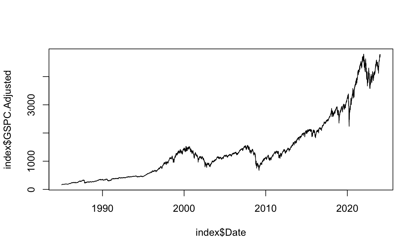

Figure 2.1: Plot of the S&P 500 Index over time starting in 1985.

The plots can be customized along many dimensions such as color and size of the labels, ticks, title, line and point type and much more. In Figure 2.2 the previous graph is customized by changing the color of the line to "orange", changing the label’s size (cex=0.5), the labels with xlab and ylab, and finally the title of the graph by setting main.

plot(index$Date, index$GSPC.Adjusted, 
     type="l", xlab="", ylab="S&P 500 Index Value (log-scale)", 
     main="S&P 500 Index", col="orange", cex.lab = 0.5)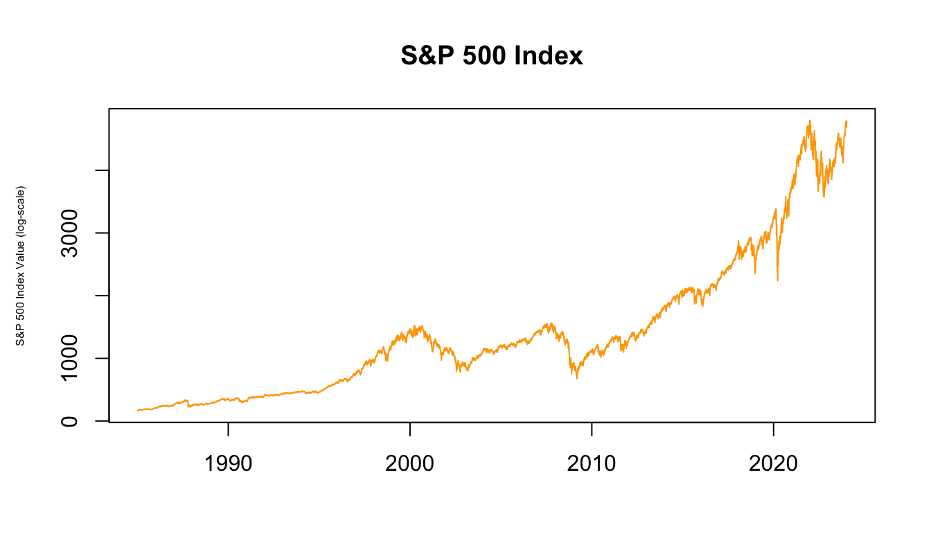

Figure 2.2: Logarithm of the S&P 500 Index at the daily frequency.

An advantage of defining time series as xts objects is that there are specialized functions to plot. For example, when we use the base function plot() on a xts object it calls a plot.xts() functions that understands the nature of the data and, among other things, sets the x-axis to the time period of the variable without the user having to specify it (as we did in the previous graph). Figure 2.3 shows the time seris plot of the adjusted closing price of the S&P 500 Index.

plot(Ad(GSPC), main="S&P 500 Index")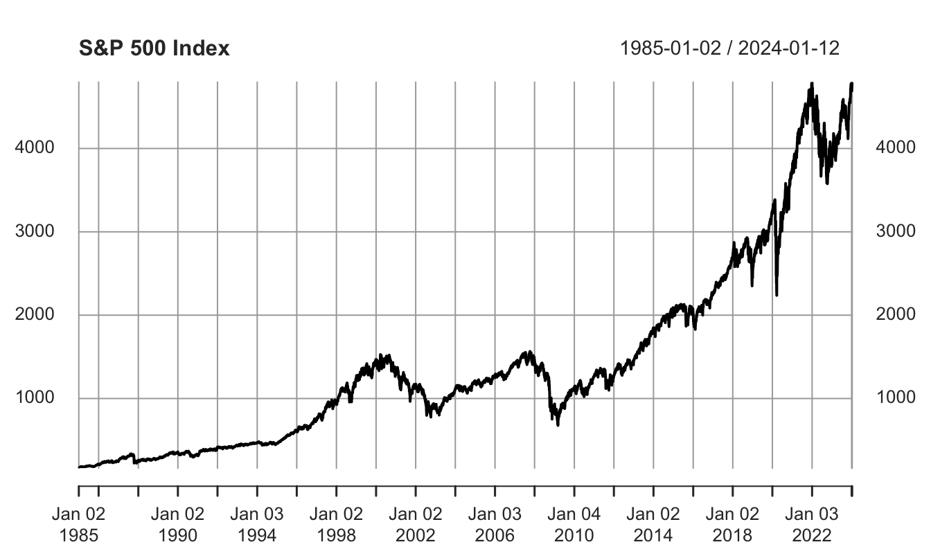

Figure 2.3: Different sub-sampling of the index.xts object.

For many economic and financial variables that display exponential growth over time, it is often convenient to plot the log of the variable rather than its level. This has the additional advantage that differences between the values at two points in time represent an approximate percentage change of the variable in that period of time. This can be achieved by plotting the natural logarithm of the variable as follows:

plot(log(Ad(GSPC)), xlab="Time",ylab="S&P 500 Index")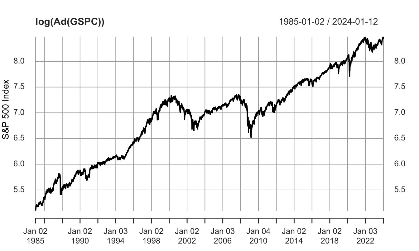

Figure 2.4: Time series plot of the logarithm of the S&P 500 Index.

There are several plotting packages in R that can be used as an alternative to the base plotting functions. I will discuss the ggplot2 package¹⁰ which is very flexible and makes it (relatively) easy to produce sophisticated graphics. This package has gained popularity among R users since it produces elegant graphs and greatly simplifies the production of advanced visualization. However, ggplot2 does not interact with xts objects so that when plotting time series we need to create a Date variable and convert the object to a data frame. This is done in the code below, where the first line produces a data frame called GSPC.df that has a column Date and the remaining columns are from the GSPC object downloaded from Yahoo Finance. The function coredata() extracts the data frame from the xts object¹¹ The ggplot2 has a qplot() function¹² that is similar to the base plot() function and requires:

• the x and y variables
• if data= is provided, then only the variable name is required
• the default plotting is points and if a different type is required it needs to be specified with geom

In the illustration below, the GSPC is converted to a data frame and then plotted using the qplot() against the date variable.

GSPC.df <- data.frame(Date = time(GSPC), coredata(GSPC))
library(ggplot2)
qplot(Date, GSPC.Adjusted, data=GSPC.df, geom="line")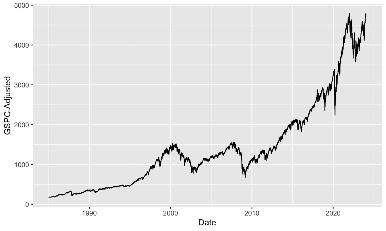

In addition to the qplot() function, the ggplot2 package provides a grammar to produce graphs. There are four building blocks to produce a graph:

• ggplot(): creates a new graph; can take as argument a data frame
• aes(): the aesthetics requires the specification of the x and y axis and the possible groups of variables
• geom_: the geometry represents the type of plot that the user would like to plot; some examples¹³:
  • geom_point()
  • geom_line()
  • geom_histogram()
  • geom_bar()
  • geom_smooth()
• theme: themes represents different styles of the graph

In Figure 2.5 there are several examples of time series plots for the S&P 500. The package ggplot2 let us save the plot in an object (plot1) which we can later plot or modify by changing some of its features (as for plot2, plot3, and plot4 below). Below I use also the function grid.arrange() from package grid.Extra to make a 2x2 grid of the 4 plots.

plot1 <- ggplot(GSPC.df, aes(Date, GSPC.Adjusted)) + geom_line(color="darkgreen")
plot2 <- plot1 + theme_bw()
plot3 <- plot2 + theme_classic() + labs(x="", y="Index", title="S&P 500")
plot4 <- plot3 + geom_line(color="darkorange") +  geom_smooth(method="lm") + 
         theme_dark() + labs(subtitle="Period: 1985/2016", caption="Source: Yahoo")
library(gridExtra)
grid.arrange(plot1, plot2, plot3, plot4, ncol=2)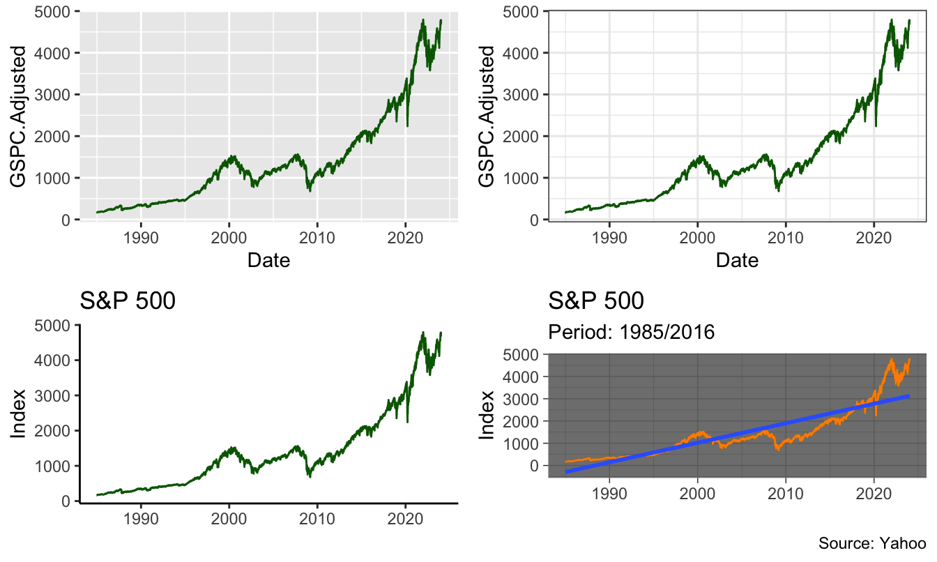

Figure 2.5: Put a caption here

A scatter plot between two variables is similarly produced by replacing the Date in the previous graphs with another variable. To produce Figure 2.6 I retrieve the returns for the S&P 500 and Nikkei 225 indices and calculate the monthly returns. The Figure shows the same scatter plot, but with different themes, labels, the geom_vline() and geom_hline() that produces vertical and horizontal lines, and the linear fit of regressing the US on the Japanese index.

data     <- getSymbols(c("^GSPC", "^N225"), from="1990-01-01")
price    <- merge(Ad(to.monthly(GSPC)), Ad(to.monthly(N225)))
ret      <- 100 * diff(log(price))
GN.df    <- data.frame(Date=time(price), coredata(merge(price,ret)))
names(GN.df) <- c("Date","SP", "NIK", "SPret","NIKret")

plot1 <- ggplot(GN.df, aes(NIKret, SPret)) + geom_point(color="red") + 
          geom_vline(xintercept = 0)  + geom_hline(yintercept = 0) 
plot2 <- plot1 + geom_smooth(method="lm", se=FALSE) + theme_bw() + 
          labs(x="NIKKEI", y="SP500") 
grid.arrange(plot1, plot2, ncol=2)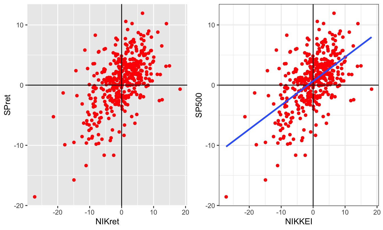

Figure 2.6: Scatter plot of the monthly returns of the NIKKEI and S&P 500 Indices.

Using the tidyquant package has the advantage that it integrates with the modern packages for plotting (ggplot2) and data wrangling (dplyr already used above). For example, a graph that would take several lines of code can be compactly customized using ggplot2. For example:

data <- tq_get(c("^GSPC", "^N225", "^STOXX50E"), 
               source = "stock.prices",  
               from="1990-01-01")

ggplot(data, aes(date, log(adjusted))) + 
  geom_line() + 
  facet_wrap(~symbol, scales = "free")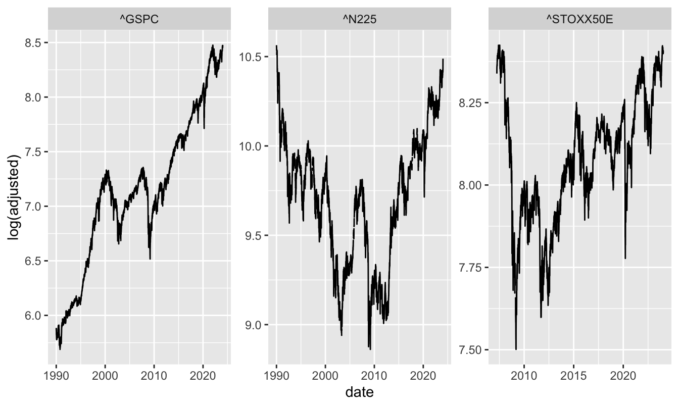

Plotting the daily percentage changes is relatively easy to do:

data <- tq_get(c("^GSPC", "^N225", "^STOXX50E"), 
               source = "stock.prices",  
               from="2000-01-01")
ret <- data %>%
        select(symbol, date, adjusted) %>%
        group_by(symbol) %>%
        mutate(ret_log = 100 * (log(adjusted) - log(lag(adjusted))))

ggplot(ret, aes(date, ret_log)) +
  geom_line() + 
  theme_bw() + 
  facet_wrap(~symbol, scale = "free")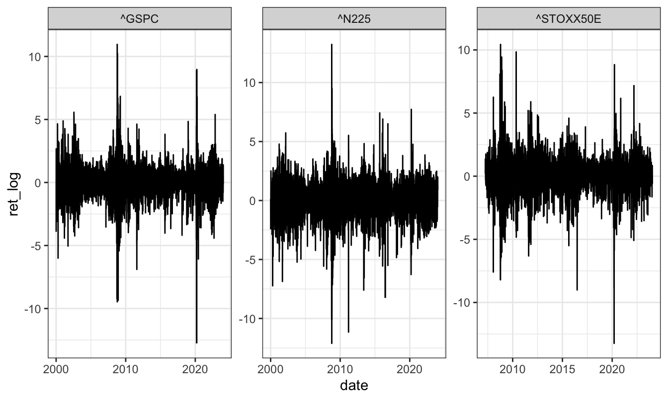

while a scatter plot of the foreign indices relative to the US index requires a few more lines of ggplot2 syntax:

sp500 = ret %>%
          filter(symbol == "^GSPC") %>% 
          ungroup() %>%
          select(date, ret_log) %>% 
          rename(sp500 = ret_log)
ret %>%
  filter(symbol != "^GSPC") %>%
  left_join(sp500, by="date") %>%
  ggplot(aes(sp500, ret_log)) + 
    geom_point(color = "red") + 
    geom_vline(xintercept = 0, linetype = "dashed") + 
    geom_hline(yintercept = 0, linetype = "dashed") + 
    geom_smooth(method = "lm", se = FALSE) + 
    facet_wrap(~symbol) + 
    theme_bw()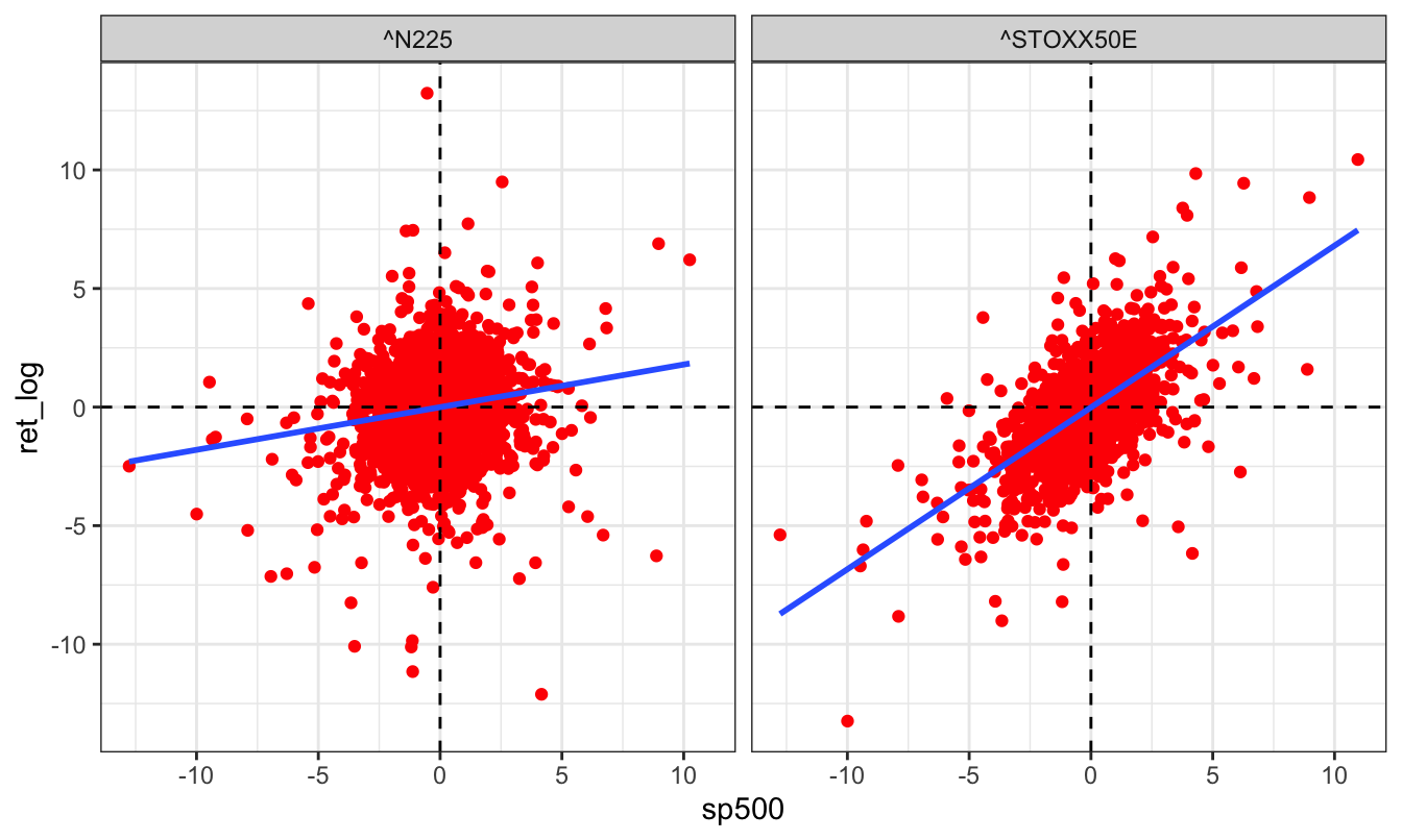

2.7 Exploratory data analysis

A first step in data analysis is to calculate descriptive statistics that summarize the main statistical features of the distribution of the data, such as the average/median returns, the dispersion, the skewness and kurtosis. A function that provides a preliminary analysis of the data is summary() that has the following output for the simple and logarithmic returns:

summary(GSPC$ret.simple)

     Index              ret.simple       
 Min.   :1990-01-02   Min.   :-11.98405  
 1st Qu.:1998-06-24   1st Qu.: -0.44911  
 Median :2006-12-31   Median :  0.05660  
 Mean   :2007-01-01   Mean   :  0.03674  
 3rd Qu.:2015-07-08   3rd Qu.:  0.57098  
 Max.   :2024-01-12   Max.   : 11.58004  
                      NA's   :1          

summary(GSPC$ret.log)

     Index               ret.log         
 Min.   :1990-01-02   Min.   :-12.76522  
 1st Qu.:1998-06-24   1st Qu.: -0.45012  
 Median :2006-12-31   Median :  0.05658  
 Mean   :2007-01-01   Mean   :  0.03019  
 3rd Qu.:2015-07-08   3rd Qu.:  0.56936  
 Max.   :2024-01-12   Max.   : 10.95720  
                      NA's   :1          

Comparing the estimates of the mean, median, and 1st and 3rd quartile (25% and 75%) for the simple and log returns shows that the values are very close. However, when we compare the minimum and the maximum the values are quite different: the maximum drop is -11.984% for the simple return and -12.765% for the logarithmic return, while the maximum gain is 11.58% and 10.957%, respectively. The reason for the difference is that the logarithmic return is an approximation to the simple return that works well when the returns are small but becomes increasingly unreliable for large (positive or negative) returns.

Descriptive statistics can also be obtained by individual commands such as mean(), sd() (standard deviation), median(), and empirical quantiles (quantile(, tau) with tau a value between 0 and 1). If there are missing values in the series we need also to add the na.rm=TRUE argument to the function in order to eliminate these values. The package fBasics contains the functions skewness() and kurtosis() that are particularly relevant in the analysis of financial data. This package provides also the function basicStats() that provides a table with all of these descriptive statistics:

library(fBasics)
basicStats(GSPC$ret.log)

                ret.log
nobs        8574.000000
NAs            1.000000
Minimum      -12.765220
Maximum       10.957197
1. Quartile   -0.450125
3. Quartile    0.569360
Mean           0.030185
Median         0.056582
Sum          258.775422
SE Mean        0.012372
LCL Mean       0.005932
UCL Mean       0.054438
Variance       1.312321
Stdev          1.145566
Skewness      -0.393862
Kurtosis      10.630710

In addition, when the analysis involves several assets we want to measure their linear dependence through measures like the covariance and correlation. For example, the my.df object defined above is composed of the US and Japanese equity index and it is interesting to measure how the two index returns co-move. The functions to estimate the covariance is cov() and the correlation is cor(), with the additional argument of use='complete.obs' that tells R to estimate the quantity for all pairs on the set of dates that are common to all assets:

Ret <- subset(GN.df, select=c("SPret","NIKret"))
cov(Ret, use='complete.obs') 

          SPret   NIKret
SPret  18.65998 14.43415
NIKret 14.43415 36.10580

The elements in the diagonal are the variances of the index returns and the off-diagonal element represents the covariance between the two series. The sample covariance is equal to 14.43 which is difficult to interpret since it depends on the scale of the two variables. That is a reason for calculating the correlation that is scaled by the standard deviation of the two variable and is thus bounded between 0 and 1. The correlation matrix is calculated as:

cor(Ret, use='complete.obs')

           SPret    NIKret
SPret  1.0000000 0.5560926
NIKret 0.5560926 1.0000000

the diagonal elements are equal to 1 because they represent the correlation of the S&P 500 (N225) with the S&P 500 (N225), while the off-diagonal element is the sample correlation between the two indices. It is equal to 0.56 which indicates that the monthly returns of the two equity indices co-move, although their correlation is not extremely high.

Another useful exploratory tool in data analysis is the histogram that represents an estimator of the distribution of a variable. Histograms are obtained by dividing the range of a variable in small bins and then count the fraction of observations that fall in each bin. The histogram plot shows the distribution characteristics of the data. The function hist() in the base package and the geom_histogram() function in ggplot2 are the commands to use in this task:

hist(GSPC$ret.log, breaks=50,  xlab="", main="")     # base function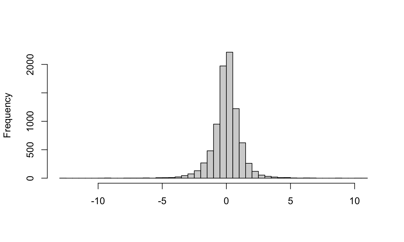

Figure 2.7: Histogram of the daily return of the SP500 produced with base graphics.

qplot(ret.log, data=GSPC, geom="histogram", bins=50) # ggplot function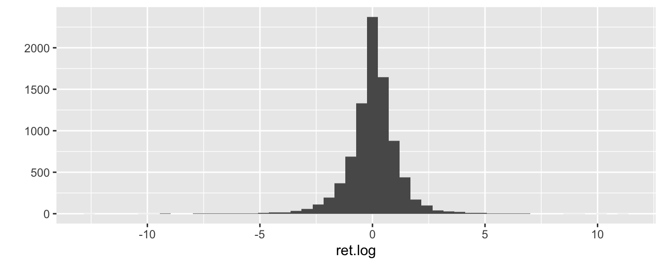

Figure 2.8: Histogram of the daily return of the SP500 produced with the ggplot2 package.

In these plots we divided the range of the variable into 50 bins and the number in the y-axis represents the number of observations. The histogram shows that daily returns are highly concentrated around 0 and with long tails, meaning that there are several observations that are far from 0 (which is approximately the mean/median of the series).

We can also add a nonparametric estimate of the frequency that smooths out the roughness of the histogram and makes the density estimates continuous¹⁴:

# base function
hist(GSPC$ret.log, breaks=50, main="", xlab="", ylab="",prob=TRUE)
lines(density(GSPC$ret.log,na.rm=TRUE),col=2,lwd=2)
box()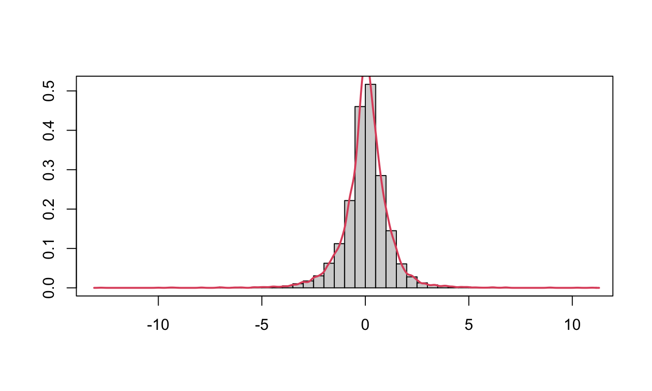

Figure 2.9: Histogram of the daily return of the SP500 produced with base graphics (left) and the ggplot2 package (right) together with a smoothed density.

# ggplot function
ggplot(GSPC, aes(ret.log)) + 
  geom_histogram(aes(y = ..density..), bins=50, color="black", fill="white") +  
  geom_density(color="red", size=1.2) + 
  theme_bw()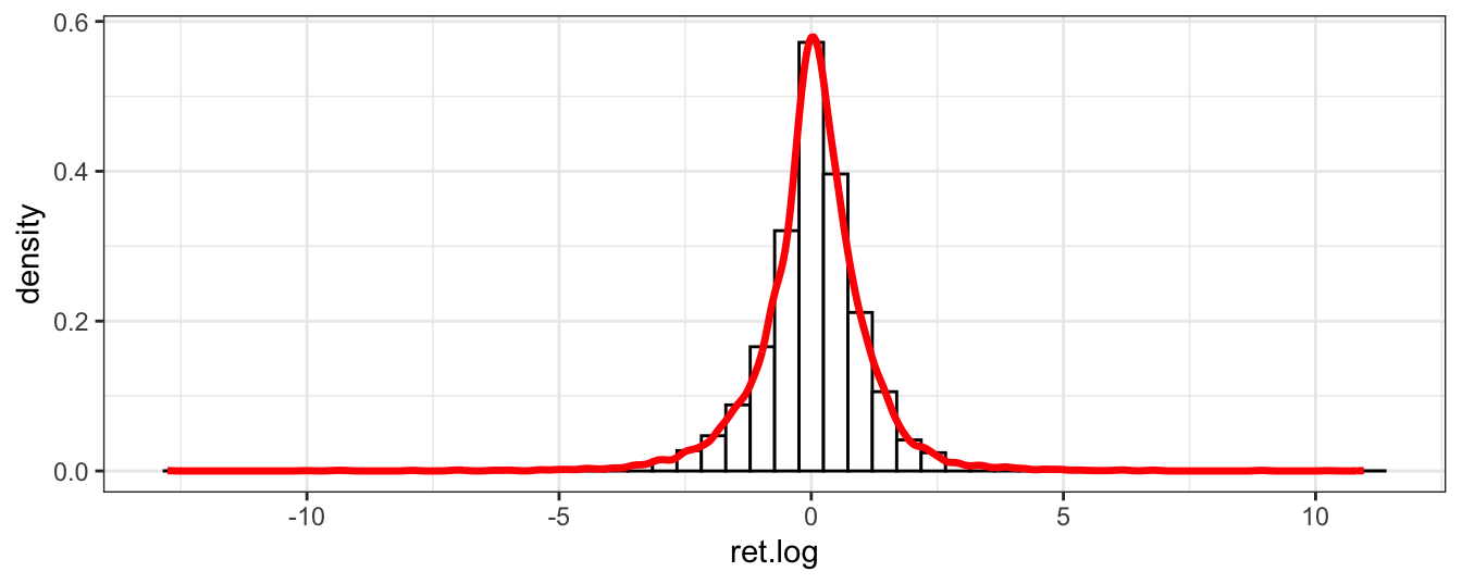

Figure 2.10: Histogram of the daily return of the SP500 produced with base graphics (left) and the ggplot2 package (right) together with a smoothed density.

2.8 Dates and Times in R

When we read a time series dataset it is convenient to define a date variable that keeps track of the time ordering of the variables. We did this already when plotting the S&P 500 when we used the command index$Date <- as.Date(index$Date, format="%Y-%m-%d"). as.Date is a command that takes a string as input and defines it of the Date type. In this case we specified the format of the variable which, in this case, is composed of a 4-digit year (%Y otherwise %y for 2-digit), a hyphen, the 2 digit month (%m), a hyphen, and finally the two digit day (%d). Other possible formats of the day is the weekday (%a abbreviate or %A unabbreviated) and month name (%b abbreviate or %B unabbreviated). The default R output is yyyy-mm-dd as shown in the examples below for different date formats:

as.Date("2011-07-17")  # no need to specify format 
as.Date("July 17, 2011", format="%B %d,%Y")
as.Date("Monday July 17, 2011", format="%A %B %d,%Y")
as.Date("17072011", format="%d%m%Y")
as.Date("11@17#07", format="%y@%d#%m")

[1] "2011-07-17"
[1] "2011-07-17"
[1] "2011-07-17"
[1] "2011-07-17"
[1] "2011-07-17"

Once we have defined dates, we can also calculate the time passed between two dates by simply subtracting two dates or using the difftime() function that allows to specify the time unit of the result(e.g., "secs", "days", and "weeks"):

date1 <- as.Date("July 17, 2011", format="%B %d,%Y")
date2 <- Sys.Date()
date2 - date1
difftime(date2, date1, units="secs")
difftime(date2, date1, units="days")
difftime(date2, date1, units="weeks")

Time difference of 4566 days
Time difference of 394502400 secs
Time difference of 4566 days
Time difference of 652.2857 weeks

In addition to the date, we might need to associate a time of the day to each observation as in the case of high-frequency data. In the previous Chapter we discussed the tick-by-tick quote data for the dollar-yen exchange rate obtained from TrueFX. The first 10 observations of the file for the month of December 2016 is shown below:

data.hf <- data.table::fread('USDJPY-2016-12.csv',
                             col.names=c("Pair","Date","Bid","Ask"),
                             colClasses=c("character","character","numeric","numeric"),
                             data.table=FALSE, verbose = FALSE, showProgress = FALSE)

      Pair                  Date     Bid     Ask
1  USD/JPY 20161201 00:00:00.041 114.682 114.691
2  USD/JPY 20161201 00:00:00.042 114.682 114.692
3  USD/JPY 20161201 00:00:00.186 114.683 114.693
4  USD/JPY 20161201 00:00:00.188 114.684 114.694
5  USD/JPY 20161201 00:00:00.189 114.687 114.696
6  USD/JPY 20161201 00:00:00.223 114.687 114.697
7  USD/JPY 20161201 00:00:00.343 114.687 114.698
8  USD/JPY 20161201 00:00:00.347 114.687 114.697
9  USD/JPY 20161201 00:00:00.403 114.687 114.695
10 USD/JPY 20161201 00:00:00.415 114.686 114.695

The first part of the date represents the day in the format yyyymmdd and we know how to handle that from the above discussion. The second part represents the time of the day the quote was issued and the format is hour:minute:second (hh:mm:ss). Notice that the seconds are decimal and 00.041 represents a fraction of a second. In this case the function as.Date() is not useful because it only takes care of the date part, but not the time part. Two other functions are available to convert date-time strings to date-time objects. The function strptime() and as.POSIXlt() can be used with similar functionality¹⁵ Both functions require to specify the format in terms of hour (%H), minute (%M), second (%S), and decimal second (%OS). Notice that the date-time produced below are defaulted to the EST time zone, but this can be easily changed with argument tz.

strptime("20161201 01:00", format="%Y%m%d %H:%M")
strptime("20161201 00:00:01", format="%Y%m%d %H:%M:%S")
strptime("20161201 00:00:00.041", format="%Y%m%d %H:%M:%OS")
as.POSIXlt("20161201 00:00:00.041", format="%Y%m%d %H:%M:%OS")

[1] "2016-12-01 01:00:00 EST"
[1] "2016-12-01 00:00:01 EST"
[1] "2016-12-01 00:00:00 EST"
[1] "2016-12-01 00:00:00 EST"

The function strptime() can also be used to define dates with no time stamp and it will produce a POSIXt date.

date1 <- as.POSIXlt("20161201 00:00:00.041", format="%Y%m%d %H:%M:%OS")
date2 <- strptime("20161201 01:15:00.041", format="%Y%m%d %H:%M:%OS")
date2 - date1
difftime(date2, date1, unit="secs")

Time difference of 1.25 hours
Time difference of 4500 secs

We can now re-define the Date column in the data.hf frame using the strptime() function:

data.hf$Date <- strptime(data.hf$Date, format="%Y%m%d %H:%M:%OS")
str(data.hf)

'data.frame':   14237744 obs. of  4 variables:
 $ Pair: chr  "USD/JPY" "USD/JPY" "USD/JPY" "USD/JPY" ...
 $ Date: POSIXlt, format: "2016-12-01 00:00:00" "2016-12-01 00:00:00" ...
 $ Bid : num  115 115 115 115 115 ...
 $ Ask : num  115 115 115 115 115 ...

2.8.1 The lubridate package

There are several packages that provide functionalities to make it easier to work with dates and times. I will discuss the lubridate package that will be used in several chapters of this book since it has an easier syntax and provides several useful functions. The package has functions that can be used to define a string as a date:

• ymd: for dates in the format year, month, day
• dmy: dates with day, month, year format
• mdy: when the format is month, day, year
• ymd_hm: in addition to the date the time is provided in hour and minute (the date part can be changed to other formats)
• ymd_hms: the time format is hour, minute, and seconds

Below are some examples of dates that are parsed with these functions¹⁶:

library(lubridate)
ymd("20170717")
ymd("2017/07/17")
ymd_hm("20170717 01:00")
ydm_hms("20171707 00:00:00.041")

[1] "2017-07-17"
[1] "2017-07-17"
[1] "2017-07-17 01:00:00 UTC"
[1] "2017-07-17 00:00:00 UTC"

Notice that ymd("17/07/2017") would output a NA with a warning message that the parsing failed. This is because the string date is in the format dmy() instead of ymd(). The package lubridate provides also a series of functions that are particularly useful to extract parts of the date-time object, as shown below:

mydate <- ydm_hms("20171707 00:00:00.041")
year(mydate)

[1] 2017

month(mydate)

[1] 7

day(mydate)

[1] 17

minute(mydate)

[1] 0

second(mydate)

[1] 0.04099989

2.9 Manipulating data using dplyr

Time series data have a major role in financial analysis and we discussed two ways to manipulate them. The first is to define the data as a time series object (e..g, xts) that consists of embedding the time series properties in the object. The alternative approach is to maintain the data as a data frame object and define a date variable that keeps track of the temporal ordering of the data.

If the second route is taken, the dplyr package¹⁷ is a useful tool that can be used to manipulate data frames. The package has the following properties:

• defines a new type of data frames, called tibble, that have some convenient features
• defines commands to manipulate data for the most frequent operations that make the task easier and more transparent
• these commands are executed faster relative to equivalent base R commands that is particularly useful when dealing with large datasets

To illustrate the use of the dplyr package I will use the GSPC.df data frame that was created earlier. It is composed of 7 columns and the last 3 rows are shown below:

           Date    Open   High     Low   Close     Volume Adjusted
9835 2024-01-10 4759.94 4790.8 4756.20 4783.45 3498680000  4783.45
9836 2024-01-11 4792.13 4798.5 4739.58 4780.24 3759890000  4780.24
9837 2024-01-12 4791.18 4802.4 4768.98 4783.83 3486340000  4783.83

The main functions (or verbs) of the dplyr package are:

• mutate: to create new variables
• select: to select columns of the data frame
• filter: to select rows based on a criterion
• summarize: uses a function to summarize columns/variables in one value
• arrange: to order a data frame based on one or more variables

In the code below, I create new variables using the mutate function. In particular, I create the percentage range calculated as 100 times the logarithm of the ratio of highest and lowest intra-day price, the open-close returns, the close-to-to close return, and a few variables that extract time information from the date using lubridate functions:

library(dplyr)
library(lubridate)

GSPC.df <- mutate(GSPC.df, range   = 100 * log(High/Low),
                           ret.o2c = 100 * log(Close/Open),
                           ret.c2c = 100 * log(Adjusted / lag(Adjusted)),
                           year    = year(Date),
                           month   = month(Date),
                           wday    = wday(Date, label=T, abbr=F))  

           Date    Open    High     Low   Close     Volume Adjusted     range
9833 2024-01-08 4703.70 4764.54 4699.82 4763.54 3742320000  4763.54 1.3676831
9834 2024-01-09 4741.93 4765.47 4730.35 4756.50 3529960000  4756.50 0.7396997
9835 2024-01-10 4759.94 4790.80 4756.20 4783.45 3498680000  4783.45 0.7248300
9836 2024-01-11 4792.13 4798.50 4739.58 4780.24 3759890000  4780.24 1.2354828
9837 2024-01-12 4791.18 4802.40 4768.98 4783.83 3486340000  4783.83 0.6983331
        ret.o2c     ret.c2c year month      wday
9833  1.2641623  1.40159454 2024     1    Monday
9834  0.3067841 -0.14789939 2024     1   Tuesday
9835  0.4927034  0.56499807 2024     1 Wednesday
9836 -0.2484161 -0.06712808 2024     1  Thursday
9837 -0.1535267  0.07506938 2024     1    Friday

Notice that the dplyr package has its own lag() and lead() functions, as well as additional functions that we will use in the following chapters. If we are interested in only a few variables of the data frame, we can use the select command with arguments the data frame and the list of variables to retain:

GSPC.df1 <- dplyr::select(GSPC.df, Date, year, month, wday, range, ret.c2c)

           Date year month      wday     range     ret.c2c
9832 2024-01-05 2024     1    Friday 0.8375644  0.18240216
9833 2024-01-08 2024     1    Monday 1.3676831  1.40159454
9834 2024-01-09 2024     1   Tuesday 0.7396997 -0.14789939
9835 2024-01-10 2024     1 Wednesday 0.7248300  0.56499807
9836 2024-01-11 2024     1  Thursday 1.2354828 -0.06712808
9837 2024-01-12 2024     1    Friday 0.6983331  0.07506938

The filter() command is used when the objective is to subset the data frame according to the values of some of the variables. For example, we might want to extract the data for the month of October 2008 (as done below), the days that are Wednesday, or that range is larger than 3. This is done by specifying the logical conditions as arguments of the filter() function:

GSPC.df2 <- dplyr::filter(GSPC.df1, year == 2008, month == 10)   # NB: the double equal sign

        Date year month      wday    range    ret.c2c
1 2008-10-01 2008    10 Wednesday 2.275859 -0.4554344
2 2008-10-02 2008    10  Thursday 4.332407 -4.1124949
3 2008-10-03 2008    10    Friday 4.946028 -1.3598566

         Date year month      wday    range   ret.c2c
21 2008-10-29 2008    10 Wednesday 5.043792 -1.114091
22 2008-10-30 2008    10  Thursday 3.672182  2.547665
23 2008-10-31 2008    10    Friday 4.126101  1.524855

Instead, the function summarize() is used to apply a certain function, such as mean() or sd(), to one or more variables in the data frame. Below, the average return and the average range is calculated for GSPC.df2 that represents the subset of the data frame for October 2008.

summarize(GSPC.df2, av.ret = mean(ret.c2c, na.rm=T), av.range = mean(range, na.rm=T))

      av.ret av.range
1 -0.8071151  6.65765

All the functions above can be combined to manipulate the data to answer the question of interest and they can also be used on groups of observations. dplyr has a function called group_by() that creates groups of observations that satisfy one or more criterion and we can then apply the summarize() function on each group. Continuing with the daily S&P 500 example, we might be interested in calculating the average return and the average range in every year in our sample. The year is thus the grouping variable that we will use in group_by() that combined with the command summarize() used earlier produces the answer:

temp <- group_by(GSPC.df1, year)
summarize(temp, av.ret = mean(ret.c2c, na.rm=T), av.range = mean(range, na.rm=T))

# A tibble: 40 × 3
    year   av.ret av.range
   <dbl>    <dbl>    <dbl>
 1  1985  0.0976     0.790
 2  1986  0.0539     1.12 
 3  1987  0.00793    1.78 
 4  1988  0.0462     1.22 
 5  1989  0.0956     0.955
 6  1990 -0.0268     1.31 
 7  1991  0.0923     1.11 
 8  1992  0.0172     0.823
 9  1993  0.0269     0.708
10  1994 -0.00616    0.821
# ℹ 30 more rows

The operations performed above can be streamlined using the piping operator %>% (read as then). This is a construct that allows to write more compact and, hopefully, more readable code. The code is more compact because it is often the case that we are not interested in storing the intermediate results (e.g., temp in the previous code chunk), but only to produce the table with the yearly average return and range. The intermediate results are passed from the operation to the left of %>% to the operation on the right or it can be referenced with a dot(.). The advantage of piping is that the sequence of commands can be structured more transparently: first mutate the variables then select some variables then group by one or more variables then summarize. The code below uses the %>% operator to perform the previous analysis and then plots the average range by year using the ggplot2 package:

GSPC.df %>% mutate(range   = 100 * log(High/Low),
                   ret.o2c = 100 * log(Close/Open),
                   ret.c2c = 100 * log(Adjusted / lag(Adjusted)),
                   year    = year(Date),
                   month   = month(Date),
                   day     = day(Date),
                   wday    = wday(Date, label=T, abbr=F)) %>%
           dplyr::select(year, range, ret.c2c) %>%
           group_by(year) %>%
           summarize(av.ret = mean(ret.c2c, na.rm=T), av.range = mean(range, na.rm=T)) %>%
           ggplot(., aes(year, av.range)) + geom_line(color="magenta") + theme_classic()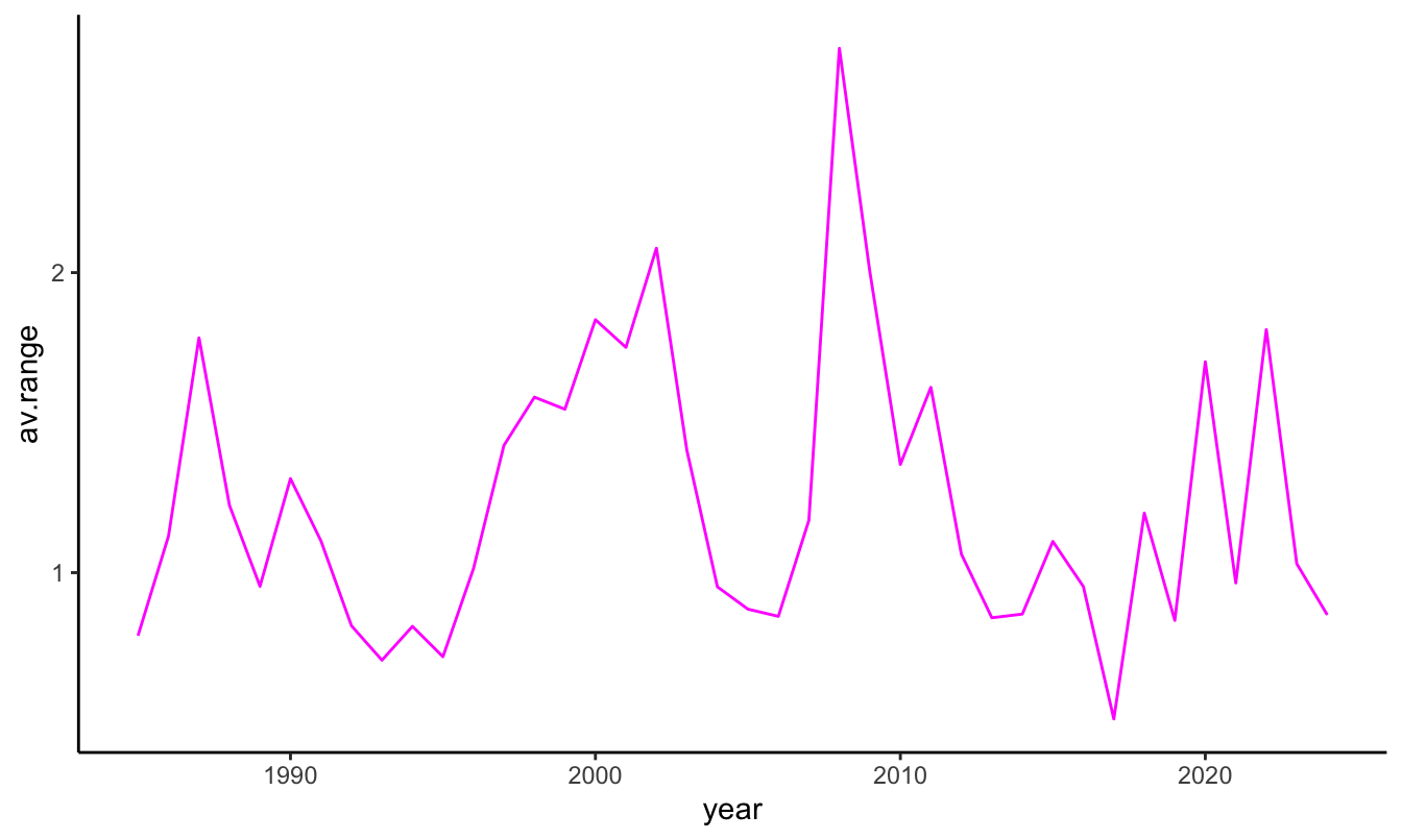 

The previous discussion demonstrates that the dplyr package is a very powerful tool to quickly extract information from a dataset with benefits that reduces the loss of flexibility deriving from time series objects. For example, let’s say that we are interested in answering the question: is volatility higher when the Index goes down relative to when it goes up? does the relationship change over time? To answer this question we need to break it down in the building blocks of the dplyr package: 1) first create a new variable that takes value, e.g., up or down (or 0 vs 1) if the GSPC return was positive or negative, 2) group the observations according to the newly created variable, 3) calculate the average range in these two groups. The R implementation is as follows:

GSPC.df1 %>% mutate(direction = ifelse(ret.c2c > 0, "up", "down")) %>%
             group_by(direction) %>%
             summarize(av.range = mean(range, na.rm=T))

# A tibble: 3 × 2
  direction av.range
  <chr>        <dbl>
1 down          1.34
2 up            1.16
3 <NA>          1.21

The results indicate that volatility, measured by the intra-day range, is on average higher in days in which the market declines relative to days in which it increases. The value for NA is due to the fact that there is one missing value in the dataset. This can be easily eliminated by filtering out NA before creating the direction variable with the command filter(GSPC.df1, !is.na(ret.c2c)). The function ifelse() used above simply assigns value up to the variable direction if the condition ret.c2c > 0 is satisfied, and otherwise it assigns the value down.

2.10 Creating functions in R

So far we discussed functions that are available in R, but one of the (many) advantages of using a programming language is that it is possible to create functions that are taylored to the analysis you are planning to conduct. We will illustrate this with a simple example. Earlier, we calculated the average monthly return of the S&P 500 Index using the command mean(GSPC$ret.log, na.rm=T) that is equal to 0.0301849. We can write a function that calculates the mean and compares the results with those of the function mean(). Since the sample mean is obtained as \(\bar{R} = \sum_{t=1}^T R_t / T\) we can write a function that takes a time series as input and gives the sample mean as output. We can call this function mymean and the syntax of defining a function is as follows:

mymean <- function(Y)
{  
  Ybar <- sum(Y, na.rm=T) / length(Y)
  return(Ybar)
}

mymean(GSPC$ret.log)

[1] 0.03018141

Not surprisingly, the result is the same as the one obtained using the mean function. More generally, a function can take several arguments, but it has to return only one outcome, which could be a list of items. The function we defined above is quite simple and it has several limitations: 1) it does not take into account that the series might have NAs, and 2) it does not calculate the mean of each column in case there are several. As an exercise, modify the mymean function to accomodate for these issues.

2.11 Loops in R

A loop consists of a set of commands that we are interested to repeat a pre-specified number of times and to store the results for further analysis. There are several types of loops, with the for loop probably the most popular. The syntax in R to implement a for loop is as follows:

for (i in 1:N)
{
   ## write your commands here
}

where i is an indicator and N is the number of times the loop is repeated. As an example, we can write a function that contains a loop to calculate the sum of a variable and compare the results to the sum() function provided in R. This function could be written as follows:

mysum <- function(Y)
{
  N    = length(Y)   # define N as the number of elements of Y
  sumY = 0           # initialize the variable that will store the sum of Y
  
  for (i in 1:N)
  {
      if (!is.na(Y[i])) sumY = sumY + as.numeric(Y[i]) # current sum is equal to previous sum 
  }                                  # plus the i-th value of Y    
  return(sumY)                       # as.numeric(): makes sure to transform 
}                                    # from other classes to a number

c(sum(GSPC$ret.log, na.rm=T), mysum(GSPC$ret.log))

[1] 258.7754 258.7754

Notice that to define the mysum() function we only use the basic + operator and the for loop. This is just a simple illustration of how the for loop can be used to produce functions that perform a certain operation on the data. Let’s consider another example of the use of the for loop that demonstrates the validity of the Central Limit Theorem (CLT). We are going to do this by simulation, which means that we simulate data and calculate some statistic of interest and repeat these operations a large number of times. In particular, we want to demonstrate that, no matter how the data are distributed, the sample mean is normally distributed with mean the population mean and variance given by \(\sigma^2/N\), where \(\sigma^2\) is the population variance and \(N\) is the sample size. We assume that the population distribution is \(N(0,4)\) and we want to repeat a large number of times the following operations:

1. Generate a sample of length N
2. Calculate the sample mean
3. Repeat 1-2 S times

Every statistical package provides functions to simulate data from a certain distribution. The function rnorm( N, mu, sigma) simulate N observations from the normal distribution with mean mu and standard deviation sigma whilst rt(N, df, ncp) generates a sample of length N from the \(t\) distribution with df degrees-of-freedom and non-centrality parameter ncp. The code to perform this simulation is as follows:

S     = 1000  # set the number of simulations       
N     = 1000   # set the length of the sample
mu    = 0      # population mean
sigma = 2      # population standard deviation

Ybar = vector('numeric', S)  # create an empty vector of S elements 
                             # to store the t-stat of each simulation
for (i in 1:S)
{
  Y        = rnorm(N, mu, sigma)  # Generate a sample of length N
  Ybar[i]  = mean(Y)              # store the t-stat 
}  
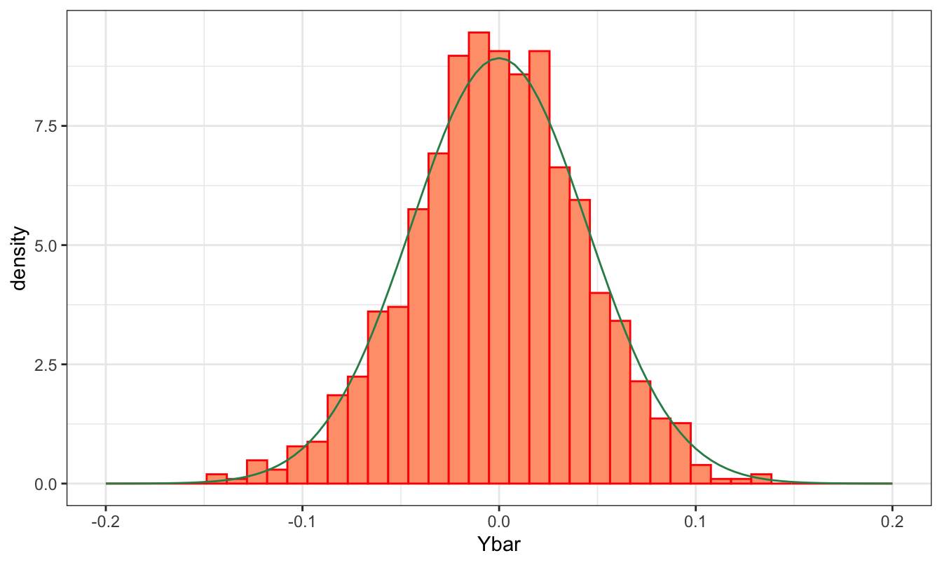
c(mean(Ybar), sd(Ybar))

[1] 0.002061413 0.061929615

The object Ybar contains 1000 elements each representing the sample mean of a random sample of length 1000 drawn from a certain distribution. We expect that these values are distributed as a normal distribution with mean equal to 0 (the population mean) and standard deviation 2/31.6227766 = 0.0632456. We can assess this by plotting the histogram of Ybar and overlap it with the distribution of the sample mean. The graph below shows that the two distribution seem very close to each other. This is confirmed by the fact that the mean of Ybar and its standard deviation are both very close to their expected values. To evaluate the normality of the distribution, we can estimate the skewness and kurtosis of store which we expect to be close to zero to indicate normality. These values are 0 and 0.03 which can be considered close enough to zero to conclude that Ybar is normally distributed.

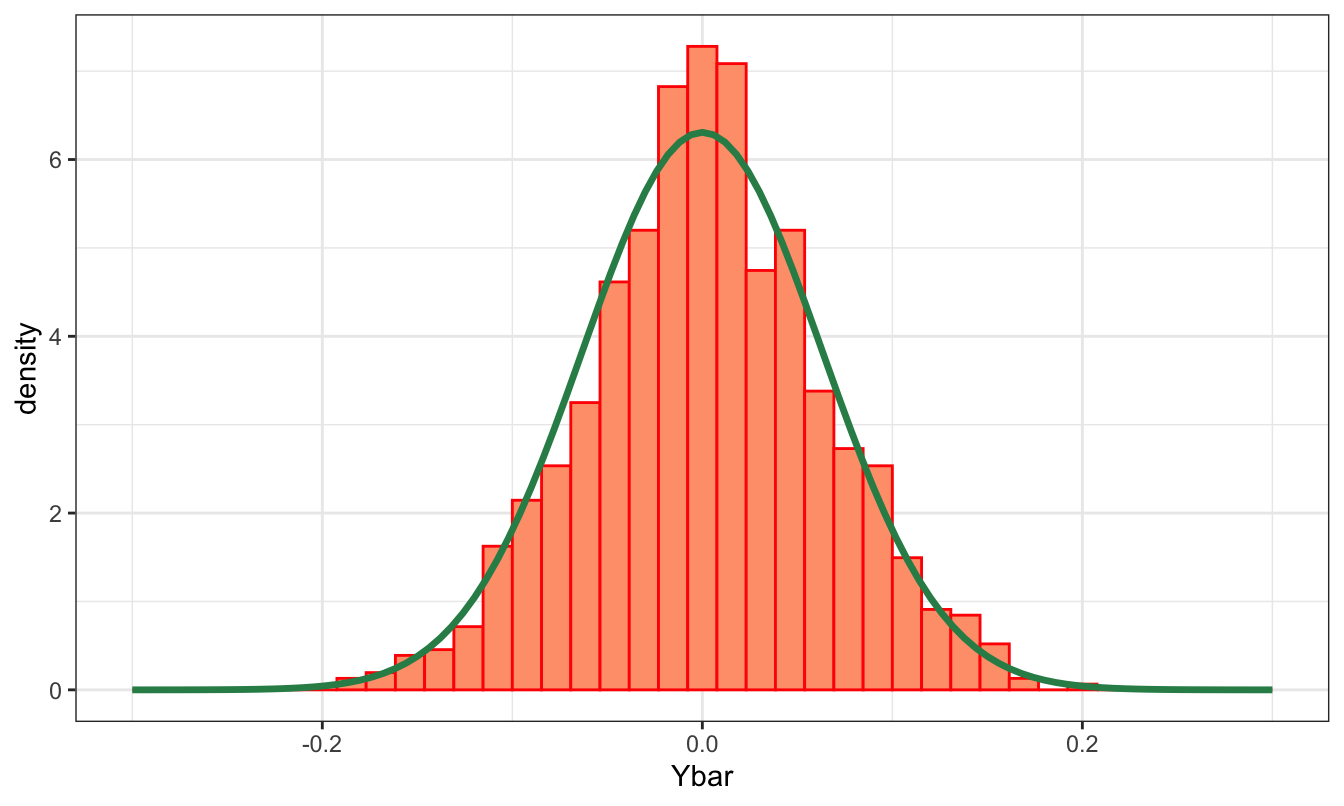
What would happen if we generate samples from a \(t\) instead of a normal distribution? For a small number of degrees-of-freedom the \(t\) distribution has fatter tails than the normal, but the CLT is still valid and we should expect results similar to the previous ones. We can run the same code as above, but replace the line Y = rnorm(N, mu, sigma) with Y = rt(N, df) with df=4. The plot of the histogram and normal distribution (with \(\sigma^2 = df / (df-2)\)) below shows that the empirical distribution of Ybar closely tracks the asymptotic distribution of the sample mean.

R commands

R functions used in this Chapter.

Ad()	day()	getSymbols()	minute()	second()	theme_bw()
apply.monthly()	density()	ggplot()	month()	select()	theme_classic()
apply.weekly()	diff()	grid.arrange()	mutate()	start()	to.monthly()
as.Date()	difftime()	group_by()	names()	str()	to.weekly()
as.POSIXlt()	end()	head()	new.env()	strptime()	window()
basicStats()	filter()	hist()	periodicity()	subset()	write.csv()
box()	fread()	labs()	plot()	sum()	xts()
class()	geom_density()	lag()	qplot()	summarize()	ydm_hms()
cor()	geom_histogram()	length()	Quandl()	summary()	year()
cov()	geom_line()	lines()	read_csv()	Sys.time()	ymd_hm()
data.frame()	geom_smooth()	merge()	read.csv()	tail()	ymd()

R packages used in this Chapter.

data.table	fBasics	gridExtra	quandl	readr
dplyr	ggplot2	lubridate	quantmod	NA

Exercises

Create a Rmarkdown file (Rmd) in Rstudio and answer each question in a separate section. To get started with Rmarkdown visit this page. The advantage of using Rmarkdown is that you can embed in the same document the R code, the output of your code, and your discussion and comments. This saves a significant amount of time relative to having to copy and paste tables and graphs from R to a word processor.

1. Perform the analysis in exercise 1 of Chapter 1 using R instead of Excel. In addition to the questions in the exercise, answer also the following question: which software between Excel and R makes the analysis easier, more transparent, more scalable, and more fun?

2. Download data from Yahoo Finance for SPY (SPDR S&P 500 ETF Trust) starting in 1995-01-01 at the daily frequency. Use the dplyr package to answer the following questions:

   • Is the daily average return and volatility (measured by the intra-day range), higher on Monday relative to Friday?
   • Which is the most volatile month of the year?
   • Is a large drop or a large increase in SPY, e.g. larger than 3% in absolute value, followed by a large return the following day? what about volatility?

3. Download data for GLD (SPDR Gold Trust ETF) and SPY (SPDR S&P 500 ETF) at the daily frequency starting in 2004-12-01. Answer the following questions:

   • Create the daily percentage returns and use the ggplot2 package to do a scatter plot of the two asset returns. Does the graph suggest that the two assets co-move?
   • Add a regression line to the previous graph with command geom_smooth(metod="lm") and discuss if it confirms your previous discussion.
   • Estimate the descriptive statistics for the two assets with command basicStats() from package fBasics; discuss the results for each asset and comparing the statistical properties of the two assets
   • Calculate the correlation coefficient between the two assets; comment on the magnitude of the correlation coefficient.
   • Use dplyr to estimate the correlation coefficient every year (instead of the full sample as in the previous question). Is the coefficient varying significantly from year to year? Use ggplot2 to plot the average correlation over time.

4. Import the TrueFX file that you used in exercise 4 of the previous Chapter. Answer the following questions:

   • Import the file using the fread() from the data.table package and the read_csv() from the readr package:
     • calculate the time that it took to load the file and compare the results
     • print the structure of the file loaded with the two functions and compare the types of the variables (in particular, the date-time variable)
   • Calculate the dimension of the data frame
   • Use dplyr to calculate the following quantities:
     • total number of quotes in each day of the sample and plot it over time
     • the intra-day range determined by the log-difference of the highest and lowest price; do a time series plot
     • create a minutes variable using the minute() function of lubridate; use group_by() and summarize() to create a price at the 1 minute interval by taking the last observation within each minute. Use ggplot2 to do a time series plot of the FX rate at the 1 minute interval.

References

Albert, Jim, and Maria Rizzo. 2012. R by Example. Springer Science & Business Media.

Wickham, Hadley. 2009. Ggplot2: Elegant Graphics for Data Analysis. Springer Science & Business Media.

Wickham, Hadley, Mine Çetinkaya-Rundel, and Garrett Grolemund. 2023. R for Data Science. " O’Reilly Media, Inc.".

Zuur, Alain, Elena N Ieno, and Erik Meesters. 2009. A Beginner’s Guide to r. Springer Science & Business Media.

---

1. The Table is obtained from this Wikipedia page. Accessed on January 16, 2024.↩︎

2. Exercise: why do we have 503 rows if the Index is composed of 500 companies? Find out.↩︎

3. See help(as.Date) for more details on this and later in the book.↩︎

4. The closing price adjusted for stock splits and dividends.↩︎

5. The function window() is more general and works for all time series objects↩︎

6. There are other functions that can be used for this task. One is the get.hist.quote() from the package tseries and the package fImport includes the yahooSeries() and fredSeries() functions. R has so many packages that there are different ways of doing almost any data analaysis task. However, for the purpose of this book I decided to stick to a few ways of doing things which I hope it is easier to learn. Once you are a proficient R programmer, you can find your way in the package jungle!↩︎

7. When downloading only one symbol, the additional argument auto.assign=FALSE assigns the data to the object data.↩︎

8. The arguments verbose and showProgress prevent the function from printing intermediate information about the reading progress. In a typical session you might want to have updates on the status of the reading, in particular when reading large files. I set the data.table argument to false because I prefer to have fread produce a data frame rather than a data.table object. The data.table package provides functionalities that are particularly useful when working with large datasets which we won’t use in this book.↩︎

9. One situation this might be useful is when different packages have functions with the same name.↩︎

10. See Wickham (2009) for more details.↩︎

11. If we did not include the coredata() part in this case the data frame would have been produced as well, but with row names represented by the dates (as in xts object). Not a big deal, though.↩︎

12. see http://docs.ggplot2.org/dev/vignettes/qplot.html for more details.↩︎

13. The complete list of geoms is available at http://docs.ggplot2.org/current/↩︎

14. The prob=TRUE argument makes the y-scale probabilities instead of frequencies↩︎

15. While the as.POSIXlt() function produces a date-time in the format year, month, day, hour, minute, and second, the function as.POSIXct() outputs a value that is the difference relative to a base date (January 1, 1970). I will discuss only as.POSIXlt() since it is the one that will be used mostly in this book.↩︎

16. The default time zone in this case is UTC rather than ETC and there is a 7-hour difference between the two time zones.↩︎

17. See the page https://cran.rstudio.com/web/packages/dplyr/vignettes/introduction.html for a more detailed introduction to the package.↩︎