3 Getting Started with Python
This Chapter introduces the main operations that we do when analyzing data, similarly to the previous chapter based on R. There are many similarities between the two languages and you should really consider to become proficient in both, as they have different strengths that are complementary and useful to exploit in data science. The reference to get started in Python is McKinney (2022) and there are plenty of other printed and online resources to learn programming in Python. Online resources include courses in Coursera, CognitiveClassAi, and Datacamp that provides online courses to get from beginner to advanced user.
3.1 Reading a local data file
The first task in a data science project is to load a dataset. A popular format for text files is comma separated values (csv) as the file List_SP500.csv that contains information about the 500 companies that are included in the S&P 500 Index1. The code below shows how to load a text file called List_SP500.csv using the read_csv() function. The pandas library is an essential tool in all aspects of data analysis, from reading a file, to wrangling with the information, and to plot the data among other tasks. In the code below we first import the library, then use the function read_csv() from pd as we called the pandas library, and finally we print the splist object which shows the first and last few rows of the data frame.
import pandas as pd
splist = pd.read_csv("List_SP500.csv")
print(splist)
Symbol Security ... Date added Founded
0 MMM 3M ... 1957-03-04 1902
1 AOS A. O. Smith ... 2017-07-26 1916
2 ABT Abbott ... 1957-03-04 1888
3 ABBV AbbVie ... 2012-12-31 2013 (1888)
4 ACN Accenture ... 2011-07-06 1989
.. ... ... ... ... ...
498 YUM Yum! Brands ... 1997-10-06 1997
499 ZBRA Zebra Technologies ... 2019-12-23 1969
500 ZBH Zimmer Biomet ... 2001-08-07 1927
501 ZION Zions Bancorporation ... 2001-06-22 1873
502 ZTS Zoetis ... 2013-06-21 1952
[503 rows x 6 columns]The next step is to check the type (e.g., strings, integer, float, and dates among others) attributed by the function to each column of the data frame splist. This can be done by appending dtypes to the splist object and the results are shown below:
splist.dtypesSymbol object
Security object
GICS Sector object
Headquarters Location object
Date added object
Founded object
dtype: objectThe information provided should be interpreted as follows:
- all variables are read of type
objectwhich is a general purpose type that can be a number, a string, or a date; it is not particularly efficient, so it is better to attribute the proper types within theread_csv()function or once the data frame is read - name of each variable included in the data frame (Symbol, Security, GICS Sector, Headquarters Location, Date added, Founded)
One type that we might want to change is the one assigned to the Date added. In this case the dates have been read as characters and we would like to define it as a date. This can be done easily using the to_datetime() functions in pandas and specifying the format of the data, in this case year-month-day:
splist['Date added'] = pd.to_datetime(splist['Date added'], format = "%Y-%m-%d")
splist.dtypes
Symbol object
Security object
GICS Sector object
Headquarters Location object
Date added datetime64[ns]
Founded object
dtype: objectLet’s consider another example. In the previous Chapter we discussed the S&P 500 Index with the data obtained from Yahoo Finance. The dataset was downloaded and saved with name GSPC.csv to a location in the disk. We can import the file in Python using the same read_csv() function introduced earlier:
sp = pd.read_csv("GSPC.csv") symbol date open ... close volume adjusted
0 ^GSPC 1995-01-03 459.209991 ... 459.109985 2.624500e+08 459.109985
1 ^GSPC 1995-01-04 459.130005 ... 460.709991 3.195100e+08 460.709991
2 ^GSPC 1995-01-05 460.730011 ... 460.339996 3.090500e+08 460.339996
3 ^GSPC 1995-01-06 460.380005 ... 460.679993 3.080700e+08 460.679993
4 ^GSPC 1995-01-09 460.670013 ... 460.829987 2.787900e+08 460.829987
... ... ... ... ... ... ... ...
7302 ^GSPC 2024-01-04 4697.419922 ... 4688.680176 3.715480e+09 4688.680176
7303 ^GSPC 2024-01-05 4690.569824 ... 4697.240234 3.844370e+09 4697.240234
7304 ^GSPC 2024-01-08 4703.700195 ... 4763.540039 3.742320e+09 4763.540039
7305 ^GSPC 2024-01-09 4741.930176 ... 4756.500000 3.529960e+09 4756.500000
7306 ^GSPC 2024-01-10 4759.939941 ... 4783.450195 3.498680e+09 4783.450195
[7307 rows x 8 columns]This is the typical format of the Yahoo Finance files that, in addition to the date, provide 6 columns that represent the opening and closing price, the intra-day high and low price, the adjusted closing price2 and the transaction volume. The structure of the object is provided here:
sp.dtypessymbol object
date object
open float64
high float64
low float64
close float64
volume float64
adjusted float64
dtype: objectIn this case all variables are classified as numerical except for the Symbol and the Date variables that are read as a strings.
3.2 Saving data files
In addition to reading files, we can also save data files to the local drive. In the example below we create a new variable in the sp data frame that represents the range. The range is one of several measures of volatility and it is defined as the percentage spread between the highest and lowest intra-day price experience by the asset. The frame is then saved with name newdf.csv using the pandas function to_csv():
sp         = pd.read_csv("GSPC.csv")
sp['date'] = pd.to_datetime(sp['date'], format="%Y-%m-%d")

# create a new variable called range
sp['Range'] = 100 * (sp['high'] - sp['low']) / sp['low']
sp.to_csv("indexdf.csv")
3.3 Time series objects
In this course we will deal exclusively with time series and it is thus convenient to explicitly define our pandas data frame as ordered in time. This can be done by set_index() of the dataframe to the time variable in the dataset, in our example the variable date. As can be seen below, once the index is set to date, the variable is not included in the dataset anymore and it is used to sort the rows of the data frame.
sp.set_index('date', inplace = True) symbol open ... adjusted Range
date ...
1995-01-03 ^GSPC 459.209991 ... 459.109985 0.452751
1995-01-04 ^GSPC 459.130005 ... 460.709991 0.690621
1995-01-05 ^GSPC 460.730011 ... 460.339996 0.337137
1995-01-06 ^GSPC 460.380005 ... 460.679993 0.657277
1995-01-09 ^GSPC 460.670013 ... 460.829987 0.441554
... ... ... ... ... ...
2024-01-04 ^GSPC 4697.419922 ... 4688.680176 0.837328
2024-01-05 ^GSPC 4690.569824 ... 4697.240234 0.841082
2024-01-08 ^GSPC 4703.700195 ... 4763.540039 1.377079
2024-01-09 ^GSPC 4741.930176 ... 4756.500000 0.742442
2024-01-10 ^GSPC 4759.939941 ... 4783.450195 0.727463
[7307 rows x 8 columns]Sometimes we might want to change the frequency of our time series. For example, converting from the daily data of the S&P 500 Index to the monthly frequency. This can be done easily with pandas using the function resample() and specifying the function used to aggregate the high-frequency observations3.
sp = sp.drop('symbol', axis = 1).resample('M').mean() open high ... adjusted Range
date ...
1995-01-31 464.721908 466.378091 ... 465.250000 0.657192
1995-02-28 481.031054 483.138950 ... 481.924737 0.646106
1995-03-31 492.570439 494.352174 ... 493.153047 0.711423
1995-04-30 507.215790 508.892633 ... 507.905791 0.639590
1995-05-31 522.969097 525.441365 ... 523.813640 0.866934
... ... ... ... ... ...
2023-09-30 4419.146484 4432.440967 ... 4409.094995 0.884435
2023-10-31 4271.700040 4296.745472 ... 4269.400945 1.281400
2023-11-30 4449.438081 4471.331938 ... 4460.063314 0.752874
2023-12-31 4675.967529 4697.617505 ... 4685.051489 0.748900
2024-01-31 4723.404297 4750.385742 ... 4733.864397 0.832169
[349 rows x 7 columns]3.4 Reading an online data file
There are many websites that provide access to economic and financial data, such as Yahoo Finance and FRED, among others. This has the advantage of being able to pull data and update previous analysis and documents (such as this notes). Most often, we will use libraries that probides ready-made function that download the data needed for the analysis. The alternative is to specify a url and downloaa the file, as shown below:
url = 'https://fred.stlouisfed.org/graph/fredgraph.csv?chart_type=line&recession_bars=on&lg_scales=&bgcolor=%23e1e9f0&graph_bgcolor=%23ffffff&fo=Open+Sans&ts=12&tts=12&txtcolor=%23444444&show_legend=yes&show_axis_titles=yes&drp=0&cosd=1999-01-01&coed=2024-08-01&height=450&stacking=&range=&mode=fred&id=EXUSEU&transformation=lin&nd=1999-01-01&ost=-99999&oet=99999&lsv=&lev=&mma=0&fml=a&fgst=lin&fgsnd=2009-06-01&fq=Monthly&fam=avg&vintage_date=&revision_date=&line_color=%234572a7&line_style=solid&lw=2&scale=left&mark_type=none&mw=2&width=1168'
data = pd.read_csv(url)
DATE EXUSEU
0 1999-01-01 1.1591
1 1999-02-01 1.1203
2 1999-03-01 1.0886
3 1999-04-01 1.0701
4 1999-05-01 1.0630
.. ... ...
295 2023-08-01 1.0910
296 2023-09-01 1.0672
297 2023-10-01 1.0565
298 2023-11-01 1.0819
299 2023-12-01 1.0909
[300 rows x 2 columns]The url above refers to the ticker EXUSEU (USD-EURO exchange rate) from January 1999 until
the most recent observation at the monthly frequency. Although passing the read_csv() function a url is possible, most often we use libraries such as the one discussed below.
3.4.1 Yahoo Finance
Yahoo Finance is a great and free resource for stock prices. The yfinance library is a popular choice for accessing data from this website. The inputs are the ticker of the stocks or indices that you want to download and the period that you are interested to obtain. In the example below we download data for the S&P500 Index (^GSPC) and Dow Jones Index (^DJI) starting in January 1990 until the most recent observation.
import yfinance as yf
data = yf.download(['^GSPC','^DJI'], start = "1990-01-01", progress = False)
The data object is a data frame that is organized by variable and, for each variable, by ticker (in case there are more than 1, as shown below):
               Adj Close               ...       Volume
                    ^DJI        ^GSPC  ...         ^DJI       ^GSPC
Date                                   ...
2024-01-10  37695.730469  4783.450195  ...  279540000.0  3498680000
2024-01-11  37711.019531  4780.240234  ...  299540000.0  3759890000
2024-01-12  37592.980469  4783.830078  ...  279250000.0  3486340000

[3 rows x 12 columns]
Accessing the adjusted closing price is quite straightforward with pandas:
data['Adj Close'] ^DJI ^GSPC
Date
1990-01-02 NaN 359.690002
1990-01-03 NaN 358.760010
1990-01-04 NaN 355.670013
1990-01-05 NaN 352.200012
1990-01-08 NaN 353.790009
... ... ...
2024-01-08 37683.011719 4763.540039
2024-01-09 37525.160156 4756.500000
2024-01-10 37695.730469 4783.450195
2024-01-11 37711.019531 4780.240234
2024-01-12 37592.980469 4783.830078
[8574 rows x 2 columns]The example above considered the case of two assets, the S&P 500 and the DJ Industrial Index. This example can be generalized to many tickers (in the example below we consider the first 10 tickers, but it could be any number):
splist      = pd.read_csv("List_SP500.csv")
ticker_list = " ".join(splist.Symbol[0:9])
data        = yf.download(ticker_list, start = "2010-01-01", progress = False)
The first three rows of the Adj Close variable is given below:
            ABBV        ABT        ACN  ...   AMD       AOS        MMM
Date                                    ...
2010-01-04   NaN  19.046156  32.455269  ...  9.70  6.033153  54.180603
2010-01-05   NaN  18.892281  32.655842  ...  9.71  5.956065  53.841270
2010-01-06   NaN  18.997196  33.003006  ...  9.57  5.958773  54.604805

[3 rows x 9 columns]
3.4.2 FRED
A very useful source of economic data is represented by the Federal Reserve Economic Data (FRED) repository that can be accessed with the fredapi library4. Also in this case you need to be able to specify the identifier (ticker) of the variable(s) that you are interested to download. In the example below, we want to download the civilian unemployment rate (UNRATE), the CPI index (CPIAUCSL), and the real GDP (GDPC1) and organize the information in a data frame:
from fredapi import Fred
import pandas as pd

fred     = Fred(api_key=my_key)

macro = {}
macro['UNRATE'] = fred.get_series('UNRATE',   observation_start = '1950-01-01')
macro['CPI']    = fred.get_series('CPIAUCSL', observation_start = '1950-01-01')
macro['GDPC1']  = fred.get_series('GDPC1',    observation_start = '1950-01-01')
macro = pd.DataFrame(macro)
UNRATE CPI GDPC1
1950-01-01 6.5 23.510 2346.104
1950-02-01 6.4 23.610 NaN
1950-03-01 6.3 23.640 NaN
1950-04-01 5.8 23.650 2417.682
1950-05-01 5.5 23.770 NaN
... ... ... ...
2023-08-01 3.8 306.269 NaN
2023-09-01 3.8 307.481 NaN
2023-10-01 3.8 307.619 NaN
2023-11-01 3.7 307.917 NaN
2023-12-01 3.7 308.850 NaN
[888 rows x 3 columns]Merging the three variables produces NA because GDPC1 is available at the quarterly frequency and UNRATE and CPIAUCSL at the monthly frequency.
3.4.3 Quandl
Quandl (now Nasdaq Data Link) works as an aggregator of public databases, but it also offer access to subscription databases. Similarly to the previously discussed sources, you will need to create an API key and know the ticker of the variables that you are interested in downloading. The Python package quandl is used in the example below to download the same series we obtained from FRED.
import quandl
quandl.read_key()

macrodata = quandl.get(['FRED/UNRATE', 'FRED/CPIAUCSL','FRED/GDPC1'], start_date = "1950-01-01")
FRED/UNRATE - Value FRED/CPIAUCSL - Value FRED/GDPC1 - Value
Date
1950-01-01 6.5 23.51 2186.365
1950-02-01 6.4 23.61 NaN
1950-03-01 6.3 23.64 NaN
1950-04-01 5.8 23.65 2253.045
1950-05-01 5.5 23.77 NaN
1950-06-01 5.4 23.88 NaN
1950-07-01 5.0 24.07 2340.112
1950-08-01 4.5 24.20 NaNThe quandl package produces an object macrodata that is already merged by date and ready for analysis.
3.4.4 Reading large files
We consider the same file used in the previous chapter about R. The dataset has 11 variables and 3,796,660 observations. The size of the file is 328Mb which is moderately large dataset, but definitely not big data. The issue with both R and Python is that the data is loaded and stored in the physical memory of the computer. This means that it is not feasible to use the commands below when the size of your dataset is larger than the phyisical memory. However, you might be in a situation where the dataset is smaller relative to the memory but the loading and processing might take longer.
The pandas function read_csv is the starting point to read the file:
import pandas as pd
import time

start_time = time.perf_counter()
crsp = pd.read_csv("./data/crsp_eco4051_jan2017.csv")
end_time = time.perf_counter()

elapsed_time = end_time - start_time
Elapsed time: 2.912313792000006The operation of loading the dataset in memory took 2.912 seconds, which is similar to the fread() and read_csv() functions in R and significantly faster than the base read.csv() function.
An alternative to the pandas function is provided by the polars library. The goal is to provide a significantly faster function that loads dataset in standard formats, such as csv. The syntax is very similar to pandas as you can see below:
import polars as pl

start_time = time.perf_counter()
crsp = pl.read_csv("./data/crsp_eco4051_jan2017.csv", ignore_errors = True)
end_time = time.perf_counter()
The read_csv() function of the polars library loads the same file we have used earlier in only 0.261, which is significantly faster than any other function we have considered so far in both R and Python. The print(crsp) function produces the following preview of the data:
shape: (3_796_660, 11)
┌────────┬────────────┬────────┬────────┬───┬───────────┬───────────┬────────┬───────────┐
│ PERMNO ┆ date       ┆ EXCHCD ┆ TICKER ┆ … ┆ PRC       ┆ RET       ┆ SHROUT ┆ ALTPRC    │
│ ---    ┆ ---        ┆ ---    ┆ ---    ┆   ┆ ---       ┆ ---       ┆ ---    ┆ ---       │
│ i64    ┆ str        ┆ i64    ┆ str    ┆   ┆ f64       ┆ str       ┆ i64    ┆ f64       │
╞════════╪════════════╪════════╪════════╪═══╪═══════════╪═══════════╪════════╪═══════════╡
│ 10000  ┆ 1985/12/31 ┆ null   ┆ null   ┆ … ┆ null      ┆ null      ┆ null   ┆ -2.5625   │
│ 10000  ┆ 1986/01/31 ┆ 3      ┆ OMFGA  ┆ … ┆ -4.375    ┆ C         ┆ 3680   ┆ -4.375    │
│ 10000  ┆ 1986/02/28 ┆ 3      ┆ OMFGA  ┆ … ┆ -3.25     ┆ -0.257143 ┆ 3680   ┆ -3.25     │
│ 10000  ┆ 1986/03/31 ┆ 3      ┆ OMFGA  ┆ … ┆ -4.4375   ┆ 0.365385  ┆ 3680   ┆ -4.4375   │
│ …      ┆ …          ┆ …      ┆ …      ┆ … ┆ …         ┆ …         ┆ …      ┆ …         │
│ 93436  ┆ 2015/09/30 ┆ 3      ┆ TSLA   ┆ … ┆ 248.39999 ┆ -0.002650 ┆ 130901 ┆ 248.39999 │
│ 93436  ┆ 2015/10/30 ┆ 3      ┆ TSLA   ┆ … ┆ 206.92999 ┆ -0.166948 ┆ 130951 ┆ 206.92999 │
│ 93436  ┆ 2015/11/30 ┆ 3      ┆ TSLA   ┆ … ┆ 230.25999 ┆ 0.112743  ┆ 130951 ┆ 230.25999 │
│ 93436  ┆ 2015/12/31 ┆ 3      ┆ TSLA   ┆ … ┆ 240.00999 ┆ 0.042343  ┆ 130951 ┆ 240.00999 │
└────────┴────────────┴────────┴────────┴───┴───────────┴───────────┴────────┴───────────┘
3.5 Transforming the data
Creating new variables in Python is easily done. When mathematical functions (e.g, logarithm) are needed for the transformation, the numpy library needs to be called. In addition, since we are working with time series, we need to take lags of the variables and the command shift(k) moves the time index back by \(k\) periods. Given that the price in period t is denoted by \(P_t\) , the simple and logarithmic returns defined as
- Simple return: \(R_t = (P_t - P_{t-1})/P_{t-1}\)
- Logarithmic return: \(r_t = log(P_t) - log(P_{t-1})\)
can be calculated as follows:
import numpy as np

GSPC = yf.download("^GSPC", start = "1990-01-01", progress = False)
GSPC['ret_simple'] = 100 * (GSPC['Adj Close'] - GSPC['Adj Close'].shift(1)) / GSPC['Adj Close'].shift(1)
GSPC['ret_log'] = 100 * (np.log(GSPC['Adj Close']) - np.log(GSPC['Adj Close'].shift(1)))
GSPC['ret_log'] = 100 * GSPC['Adj Close'].pct_change()
Notice that the pandas library has already the pct_change() method to calculate the logarithmic return or percentage change. When dealing with several stocks, the transformation to logarithmic returns is quite efficiently done with just one command:
data = yf.download("^GSPC ^N225 ^STOXX50E", start = "2000-01-01", progress = False)
ret  = 100 * data['Adj Close'].pct_change()
^GSPC ^N225 ^STOXX50E
Date
2024-01-12 0.075098 1.504286 0.849569
2024-01-15 0.000000 0.912608 -0.565619
2024-01-16 0.000000 -0.787174 -0.5771453.6 Plotting the data
There are two main Python libraries for visualization. matplotlib allows more sophisticated plotting but requires more user involvement in customizing the graph. On the other hand, seaborn has many out-of-the-shelf functions to satisfy the majority of plotting needs while wrangling and exploring a dataset. In addition, pandas data frames have built-in functions for quickly plotting the data. We will explore these three options to get started plotting, sorry, visualizing data.
In the code below, we first download from Yahoo Finance data for the S&P 500 Index starting in January 1990 at the daily frequency. We then select the Close column of the pandas data frame and plot it, including some matplotlib customization of the axis labels and title.
import matplotlib.pyplot as plt

sp = yf.download("^GSPC", start = "1990-01-01", progress = False)
sp['Close'].plot()
plt.xlabel("Date")
plt.ylabel("Adjusted")
plt.title("S&P500 Index")
plt.show()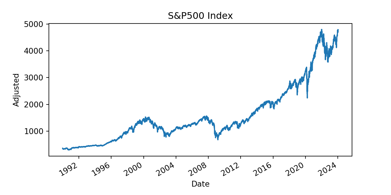
(#fig:py_ch1fig1)Plot of the S&P 500 Index over time starting in 1985.
Macroeconomic and financial variables have the tendency to grow at an exponential rate and the logarithmic transformation is typically applied to approximately linearize the increasing trend. This is done in the example below:
np.log(sp['Close']).plot()
plt.xlabel("Date")
plt.ylabel("Adjusted")
plt.title("S&P500 Index")
plt.show()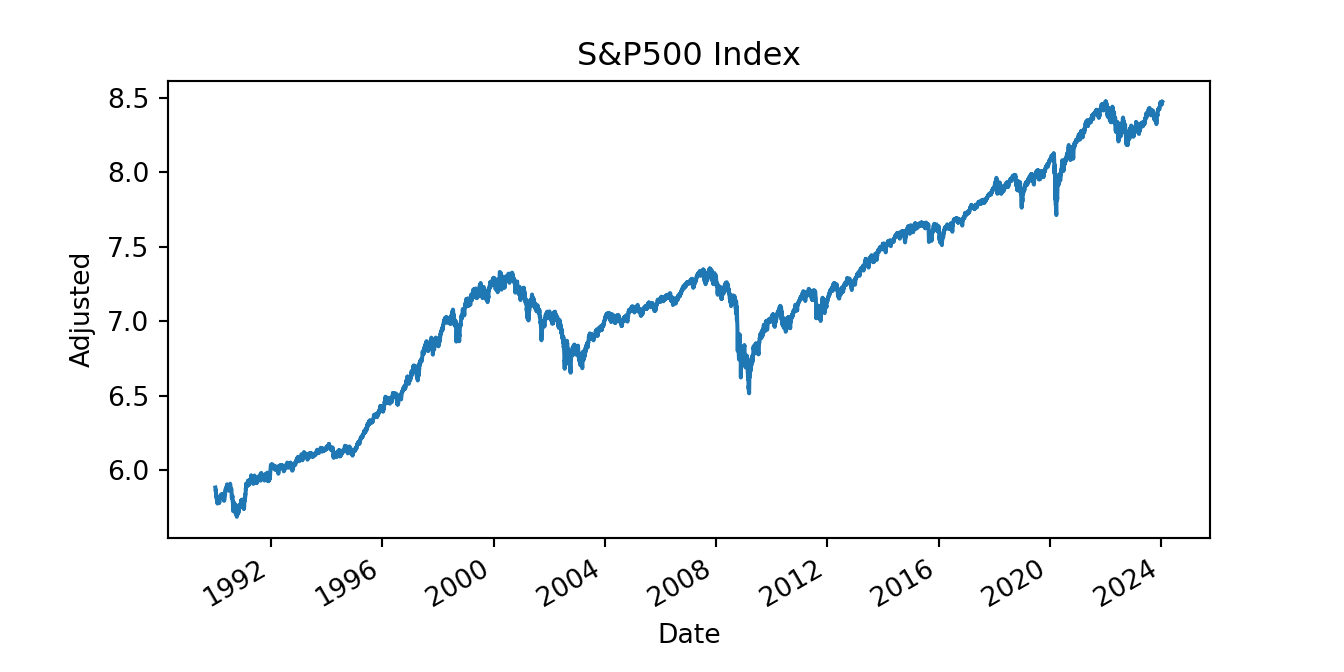
When there are two or more variables involved in the analysis, the goal is often to understand their co-movement. Plotting the time series as shown below might not be very helpful as they overlap and it is difficult to distinguish the variation of the two variables.
data = yf.download('^GSPC ^N225', start = "1990-01-01", progress = False)
ret = 100 * data['Adj Close'].pct_change().dropna()
ret = ret.resample('M').mean()

ret.plot()
plt.show()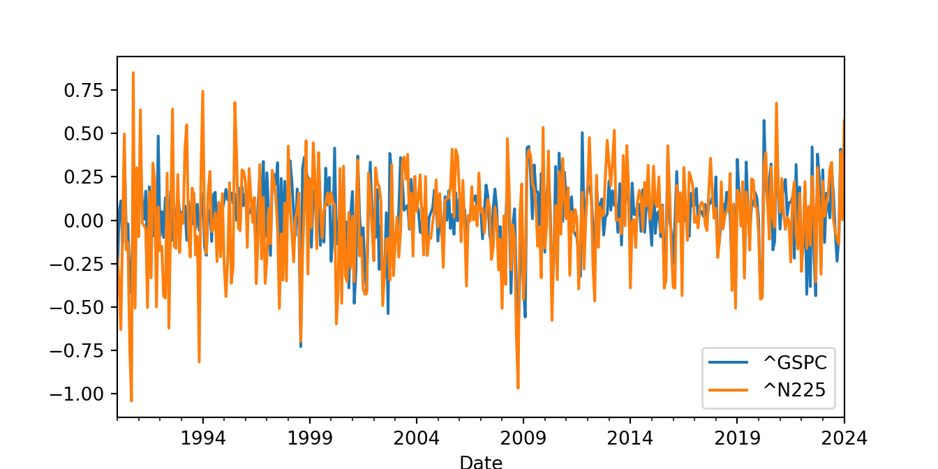
An alternative is to plot the variables in separate panels using matplotlib as shown below:
fig = plt.figure()
ax1 = fig.add_subplot(121)
ax2 = fig.add_subplot(122)
ax1.plot(ret['^GSPC'])
ax1.set_title("S&P 500")
ax2.plot(ret['^N225'])
ax2.set_title("NIKKEI")
plt.tight_layout()
plt.show()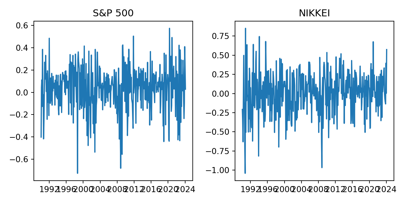
The best way to visually assess the dependence between two variables is to draw a scatter plot. Below are three ways of doing this, either using the matplotlib and seaborn libraries, or using the scatter() function in the pandas library. In these graphs, we also plot a regression line to have a more precise idea of the linear relationship between the variables, in this case the S&P 500 and NIKKEI returns.
First, using matplotlib:
import numpy as np

fig = plt.figure()
plt.scatter(ret['^N225'], ret['^GSPC'], color = "red", s = 10)
plt.axvline(x = 0, color = 'black')
plt.axhline(y = 0, color = 'black')
plt.xlabel("NIKKEI")
plt.ylabel("S&P 500")
b1, b0 = np.polyfit(ret['^N225'], ret['^GSPC'], deg = 1)
xseq = np.linspace(ret['^N225'].min(), ret['^N225'].max(), num=10)
plt.plot(xseq, b0 + b1 * xseq, '-',lw = 2)
plt.show()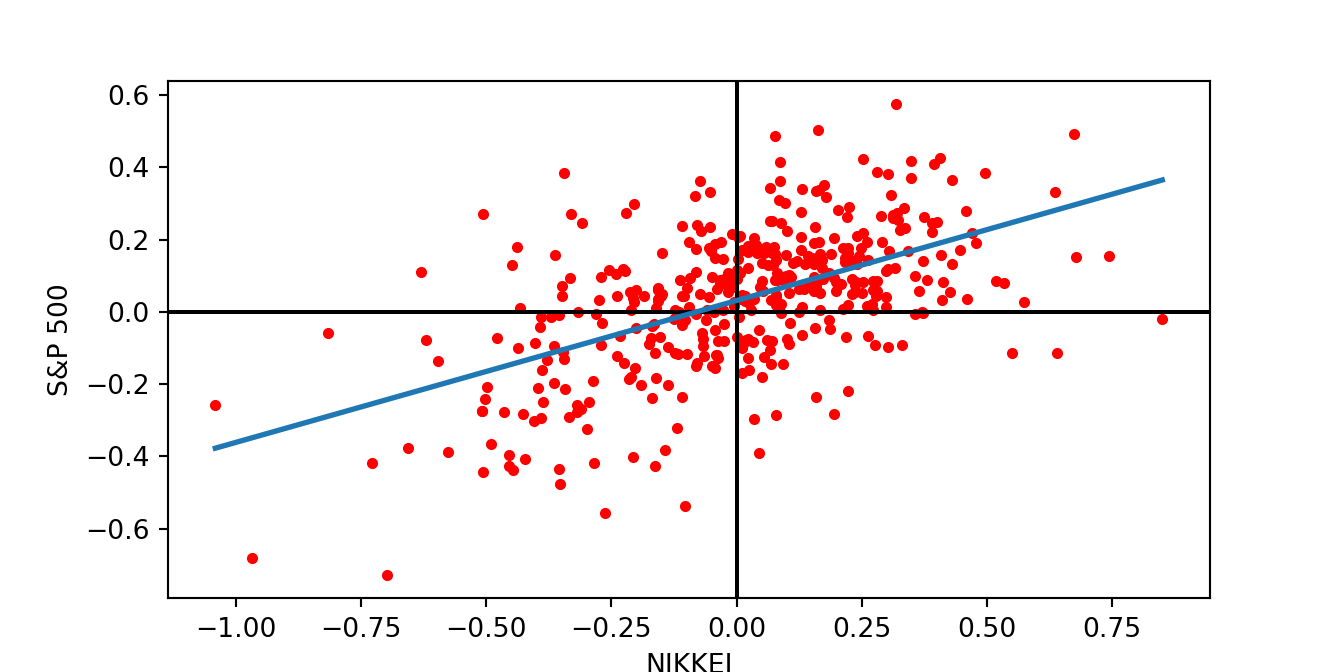
Then, using seaborn and notice how compact the code is:
import seaborn as sns

sns.regplot(x='^N225',y='^GSPC',data=ret, fit_reg=True, ci = None,
            color="red",  line_kws=dict(color="black"))
plt.axvline(x = 0, color = 'black')
plt.axhline(y = 0, color = 'black')
plt.show()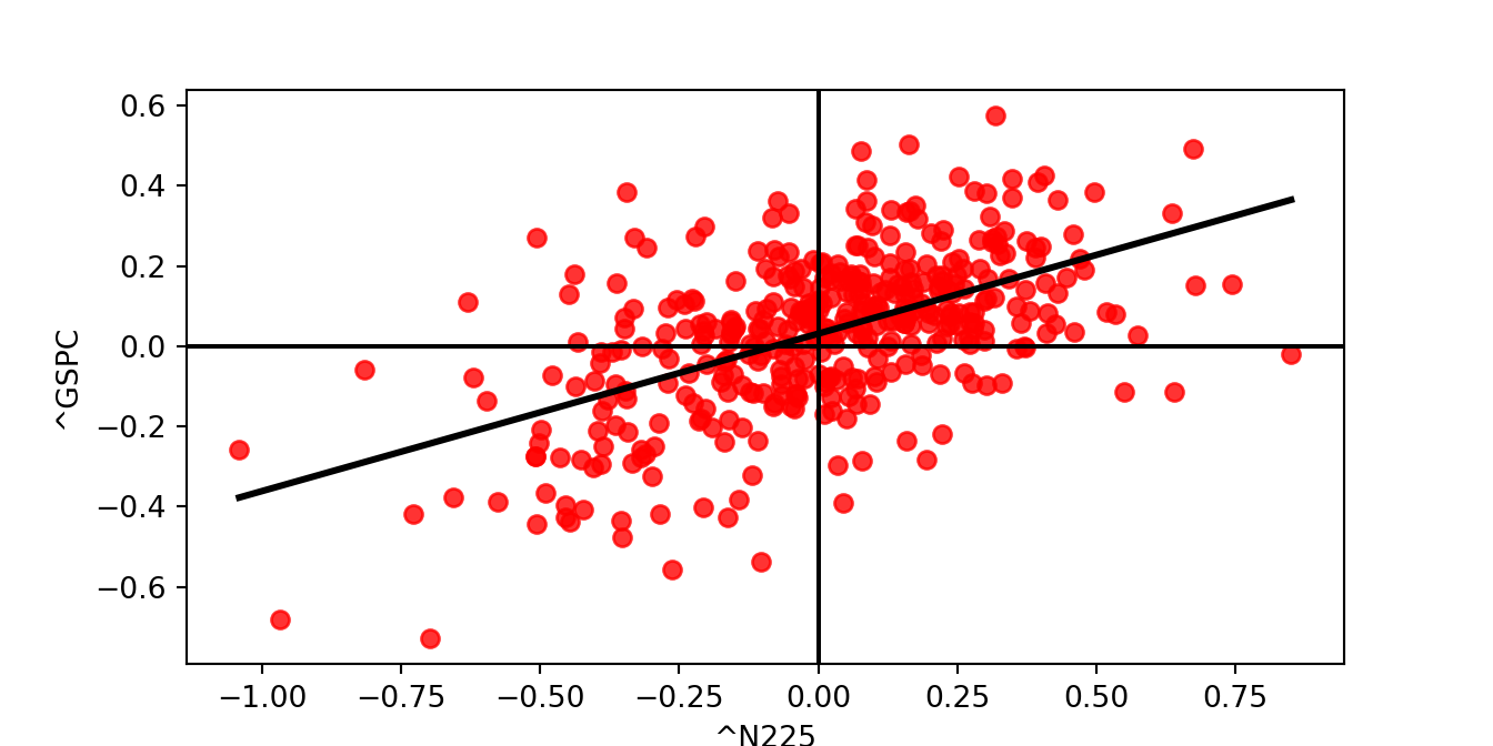
And finally, using the pandas function:
ret.plot.scatter("^N225", "^GSPC", s=10, color = "red")
plt.axvline(x = 0, color = 'black')
plt.axhline(y = 0, color = 'black')
#plt.xlabel("NIKKEI")
#plt.ylabel("S&P 500")
b1, b0 = np.polyfit(ret['^N225'], ret['^GSPC'], deg = 1)
xseq = np.linspace(ret['^N225'].min(), ret['^N225'].max(), num=10)
plt.plot(xseq, b0 + b1 * xseq, '-',lw = 2)
plt.show()
3.7 Exploratory data analysis
Estimating summary statistics in Python is as simple as in R and with very similar syntax. The describe() method is a first approach that calculates the most relevant statistics for each column of the data frame:
GSPC.describe() Open High ... ret_simple ret_log
count 8574.000000 8574.000000 ... 8573.000000 8573.000000
mean 1586.879857 1596.268336 ... 0.036743 0.036743
std 1093.550212 1099.428716 ... 1.143899 1.143899
min 295.450012 301.450012 ... -11.984055 -11.984055
25% 895.752487 906.320007 ... -0.449114 -0.449114
50% 1268.224976 1276.195007 ... 0.056598 0.056598
75% 2051.219971 2063.415039 ... 0.570984 0.570984
max 4804.509766 4818.620117 ... 11.580037 11.580037
[8 rows x 8 columns]We might also be interested in estimating summary statistics individually, and some examples are provided below:
GSPC.ret_log.mean()0.03674340978785547GSPC.ret_log.median()0.05659803737392277GSPC.ret_log.std()1.1438989492442115GSPC.ret_log.quantile(0.25)-0.4491138911119963GSPC.ret_log.quantile(0.75)0.5709842747752214GSPC.ret_log.max()11.580036951513705GSPC.ret_log.min()-11.984055240393443Notice that we do not need to specify any argument related to missing values (the na.rm = TRUE in R) as they are by default dismissed.
While the correlation is
ret.cov() ^GSPC ^N225
^GSPC 0.038795 0.029531
^N225 0.029531 0.075193The elements in the diagonal are the variances of the index returns and the off-diagonal element represents the covariance between the two series. The sample covariance is equal to 0.03 which is difficult to interpret since it depends on the scale of the two variables. That is a reason for calculating the correlation that is scaled by the standard deviation of the two variable and is thus bounded between 0 and 1. The correlation matrix is calculated as:
ret.corr() ^GSPC ^N225
^GSPC 1.000000 0.546757
^N225 0.546757 1.000000The correlation between the monthly returns of the two indices is 0.547 which indicates a co-movement between the two markets. This is expected since global equity markets react to common news of global relevance (e.g., the price of oil) although the correlation is not perfect due to country-specific news that affect only one of the indices.
The distribution of the data can be visualized by the histogram of the data. The easiest way to do this is via the hist() method of the pandas data frame:
import matplotlib.pyplot as plt

ret.hist(bins = 50)
array([[<AxesSubplot: title={'center': '^GSPC'}>,
<AxesSubplot: title={'center': '^N225'}>]], dtype=object)plt.show()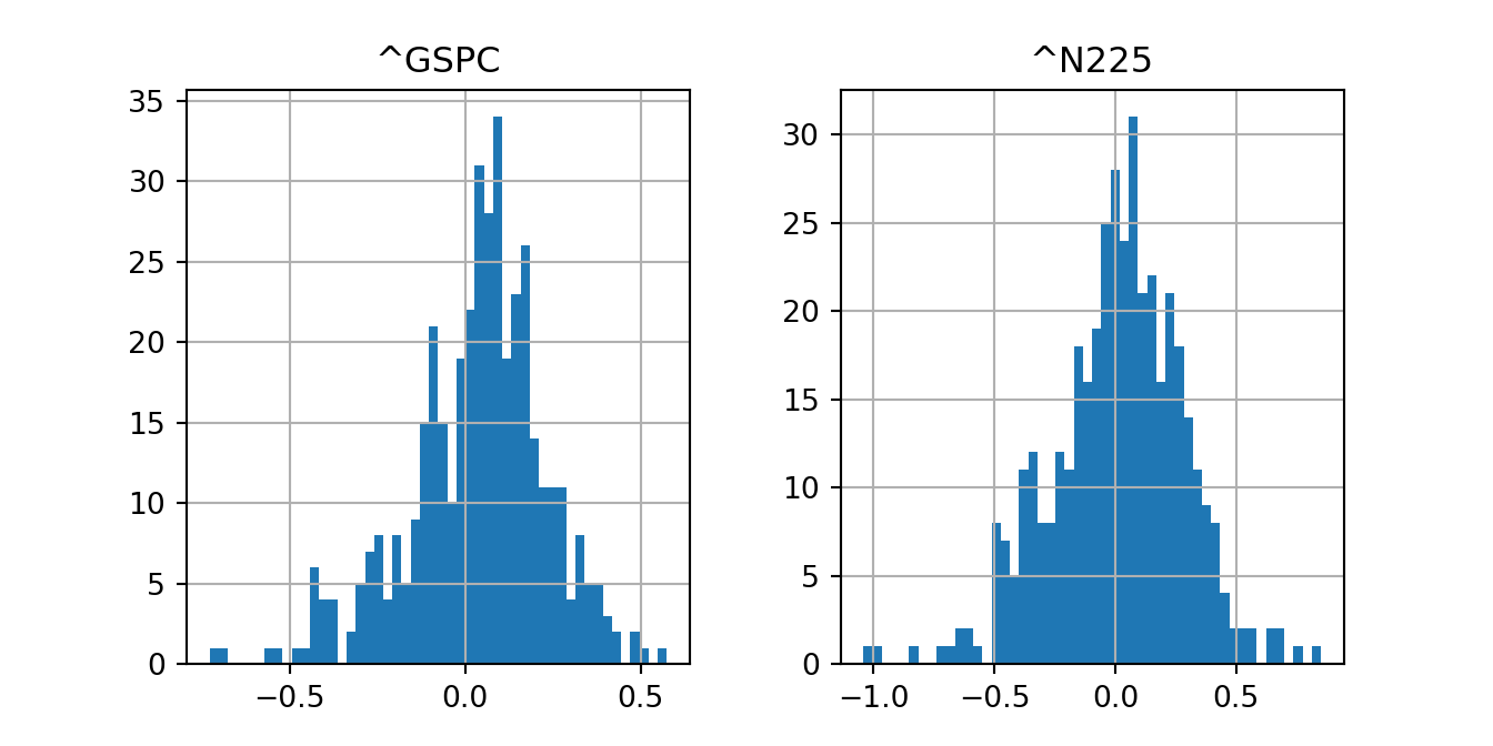
Adding to the histogram a non-parametric density estimate is easily done in seaborn as follows:
import seaborn as sns

sns.histplot(GSPC.ret_log, kde=True, bins=50)
plt.show()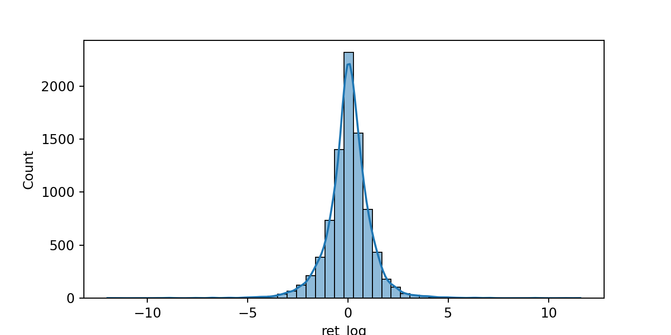
3.8 Dates and Times in Python
The ability to handle different formats of dates and times is an important characteristic of both Python and R. The datetime library provides the strptime() function that converts strings to a date-time type.
from datetime import datetime

# as.Date("2011-07-17")
print(datetime.strptime("2011-07-17", "%Y-%m-%d").date())
print(datetime.strptime("July 17, 2011", "%B %d, %Y").date())
print(datetime.strptime("Monday July 17, 2011", "%A %B %d, %Y").date())
print(datetime.strptime("17072011", "%d%m%Y").date())
2011-07-17
2011-07-17
2011-07-17
2011-07-17Operations with dates can be done easily and formatted in different units (e.g., seconds, days, etc):
from datetime import datetime, timedelta

date1 = datetime.strptime("July 17, 2011", "%B %d, %Y")
date2 = datetime.today()

# Difference in seconds
seconds_difference = (date2 - date1).total_seconds()
print("Difference in seconds:", seconds_difference)
Difference in seconds: 394527292.27172# Difference in days
days_difference = (date2 - date1).days
print("Difference in days:", days_difference)Difference in days: 4566When using intra-day price data, either from equity or FX markets, the time component is very important as there are typically several trades and quotes within a second. So, in this cases we need also to be able to handle this type of time units. As an example, below we load a file that provides bid and ask prices for the USD/JPY exchange rate for the month of December 2016.
import pandas as pd

fx = pd.read_csv('./TrueFXdata/USDJPY-2016-12.csv',
                names = ["Pair","Date","Bid","Ask"])
print(fx)
Pair Date Bid Ask
0 USD/JPY 20161201 00:00:00.041 114.681999 114.691002
1 USD/JPY 20161201 00:00:00.042 114.681999 114.692001
2 USD/JPY 20161201 00:00:00.186 114.682999 114.693001
3 USD/JPY 20161201 00:00:00.188 114.683998 114.694000
4 USD/JPY 20161201 00:00:00.189 114.686996 114.695999
... ... ... ... ...
14237739 USD/JPY 20161230 21:59:55.646 116.929001 117.061996
14237740 USD/JPY 20161230 21:59:55.761 116.929001 117.061996
14237741 USD/JPY 20161230 21:59:56.195 116.929001 117.111000
14237742 USD/JPY 20161230 21:59:56.312 116.838997 117.111000
14237743 USD/JPY 20161230 21:59:56.322 116.821999 117.094002
[14237744 rows x 4 columns]The column Date is imported as a string and we need to convert it to a datetime format to define it as a time series. The first quote recorded refers to December 1st, 2016, at hour 00, minute 00, and second 00.041, that is, 41 milliseconds. One millisecond later there was another quote that changed slightly the ask price but not the bid price. To handle the situation in which we have observations at the millisecond frequency, we need to specify the format of the datetime as follows:
print(datetime.strptime("20161201 00:00:00.041", "%Y%m%d %H:%M:%S.%f"))2016-12-01 00:00:00.041000where the time part uses %Hto define the hours, %M the minutes, and %S.%f is used for the microseconds. Using %S would assume that seconds are from 00 to 59 and do not contains milliseconds. Below are some example of when using the different specification of the format:
from datetime import datetime

print(datetime.strptime("20161201 01:00", "%Y%m%d %H:%M"))
2016-12-01 01:00:00print(datetime.strptime("20161201 00:00:01", "%Y%m%d %H:%M:%S"))2016-12-01 00:00:01Back to the USD/JPY dataset, we can define the Date column using the strptime() function and taking into account the milliseconds of the quotes:
fx['Date'] = pd.to_datetime(fx['Date'], format="%Y%m%d %H:%M:%S.%f")
print(fx.dtypes)
Pair object
Date datetime64[ns]
Bid float64
Ask float64
dtype: objectThe Date is now of type datetime64 as intended. We could also set the Date as the index of the data frame and plot the mid-point between bid and ask prices:
fx.set_index('Date', inplace = True)
fx['Mid'] = (fx['Bid'] + fx['Ask']) / 2
fx['Mid'].plot()
plt.show()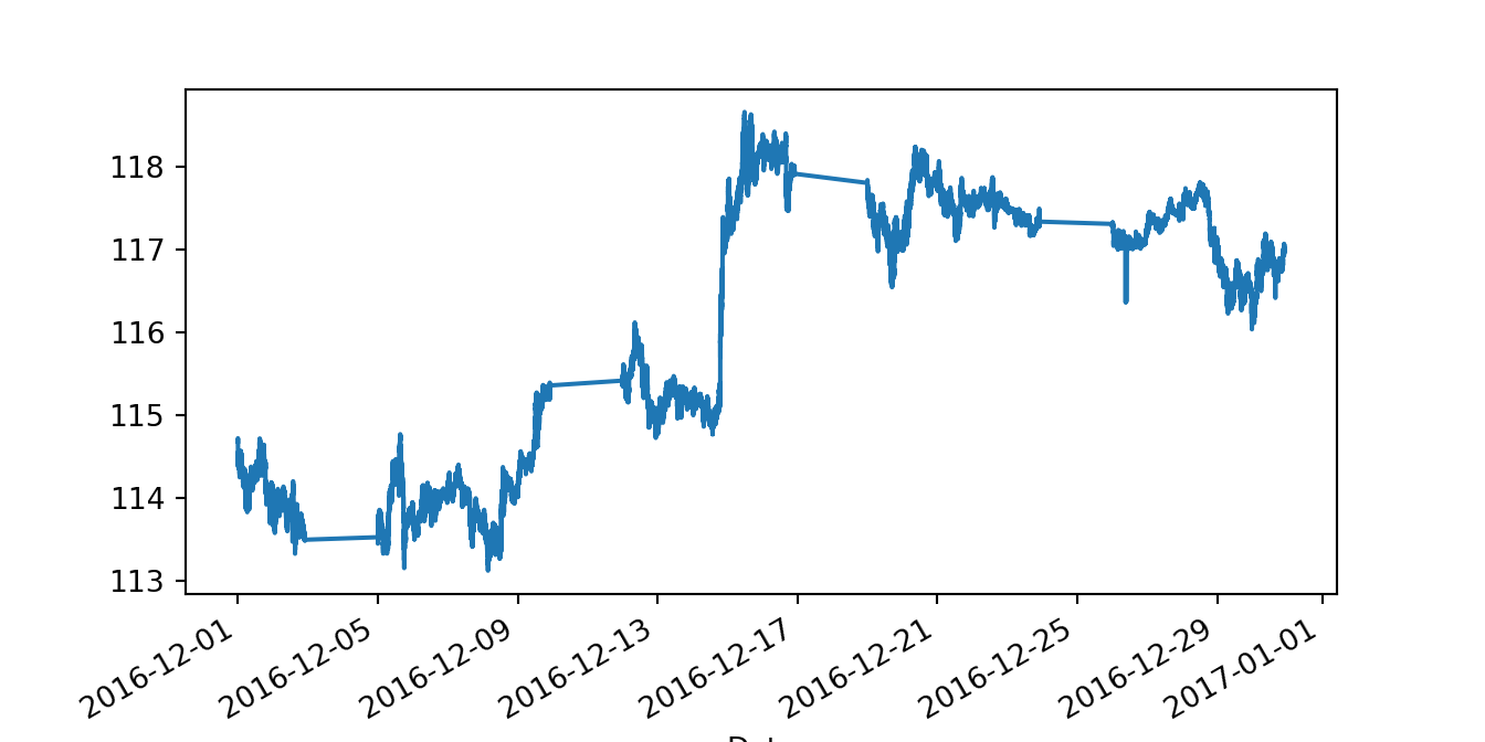
3.9 Manipulating data
Creating new variables as transformations of existing variables in a data frame is quite straightforward. Sometimes it is also useful to create new variables that represent the year or month of the observations (for grouping purposes as shown further down). In the example below we create the following variables:
range: intra-day range define as the log-difference of the highest and lowest intra-day pricesret.o2c: open-to-close returnret.o2c: open-to-close returnret.c2c: close-to-close returnyear: the year the observation refers tomonth: extracts the month of the observation (numeric)day: the day of the month (numeric)wday: day of the week (string)
GSPC['range'] = 100 * np.log(GSPC['High'] / GSPC['Low'])
GSPC['ret.o2c'] = 100 * np.log(GSPC['Close'] / GSPC['Open'])
GSPC['ret.c2c'] = 100 * np.log(GSPC['Adj Close'] / GSPC['Adj Close'].shift(1))
GSPC['year'] = pd.DatetimeIndex(GSPC.index).year
GSPC['month'] = pd.DatetimeIndex(GSPC.index).month
GSPC['day'] = pd.DatetimeIndex(GSPC.index).day
GSPC['wday'] = pd.DatetimeIndex(GSPC.index).day_name()
range ret.o2c ret.c2c year month day wday
Date
1990-01-02 2.166817 1.764201 NaN 1990 1 2 Tuesday
1990-01-03 0.751585 -0.258889 -0.258889 1990 1 3 Wednesday
1990-01-04 1.649723 -0.865030 -0.865030 1990 1 4 Thursday
1990-01-05 1.222048 -0.980414 -0.980414 1990 1 5 Friday
1990-01-08 1.049977 0.450431 0.450431 1990 1 8 Monday
... ... ... ... ... ... ... ...
2024-01-08 1.367683 1.264162 1.401595 2024 1 8 Monday
2024-01-09 0.739700 0.306784 -0.147899 2024 1 9 Tuesday
2024-01-10 0.724830 0.492703 0.564998 2024 1 10 Wednesday
2024-01-11 1.235483 -0.248416 -0.067128 2024 1 11 Thursday
2024-01-12 0.698333 -0.153527 0.075069 2024 1 12 Friday
[8574 rows x 7 columns]A frequent manipulation task to perform on a dataset is to aggregate data based on different pre-defined groups. For example, we might be interested in calculating the average monthly range as in the example below:
GSPC_year = GSPC[['year', 'range']].groupby('year').agg(av_range=('range', 'mean')).reset_index()The groupby() command separates the observations based on the different values of the grouping variable (year in the example). Then, to each group the agg() function perform an operation (mean()) that typically results in a scalar value.
GSPC_year.tail(3) year av_range
32 2022 1.810140
33 2023 1.029442
34 2024 0.859224Let’s plot the annual average range (or volatility) in the sample period considered:
plt.plot(GSPC_year['year'], GSPC_year['av_range'], color='magenta')
plt.xlabel('Year')
plt.ylabel('Average Range')
plt.title('Average Range over Years')
plt.show()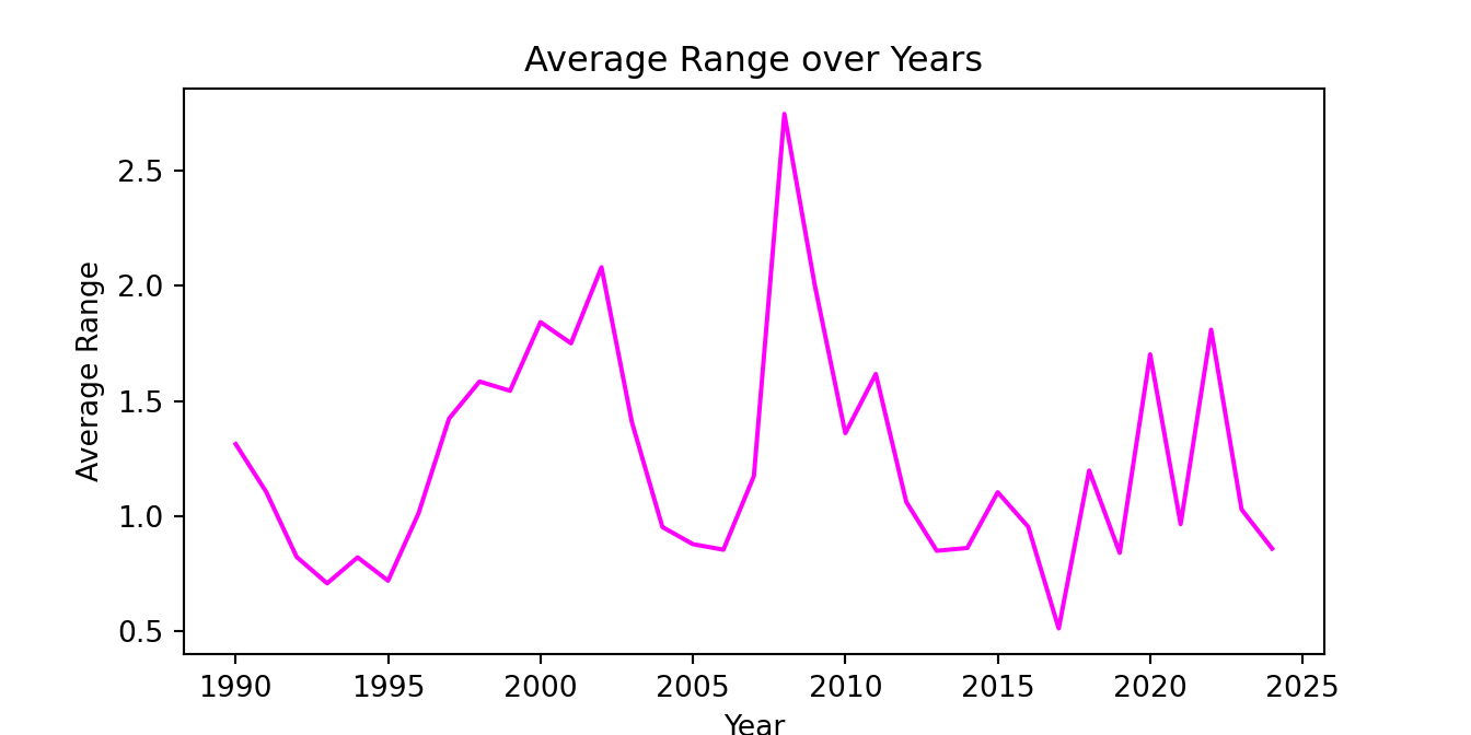
3.10 Creating functions in Python
The ability to create new functions is an important aspect of programming languages such as R and Python. A typical use case is a set of operations that need to be applied repetitively and for which no pre-define function exists. In this case the user can define a new function that take one of more inputs, performs a set of operations on the inputs, and then outputs the outcome. The example below shows how to define a function called mymean() that calculates the sample average of a vector of data Y. We have already used the predefined function mean() to calculate the average, which provides a benchmark to evaluate our mymean() function works correctly.
A function starts with a def statement followed by the name of the function and the list of inputs of the function. The definition is then followed by a set of operation on the inputs which ends with a return statement which defines the output of the function, in the this case \(\overline{Y}\) the sample average.
def mymean(Y):
    Y    = Y.dropna()
    Ybar = sum(Y) / len(Y)
    return Ybar
Let’s calculate the average return of the S&P 500 using the mymean() and mean() functions:
average1 = mymean(GSPC.ret_log)
average2 = GSPC['ret_log'].mean()
print(np.round(average1,7), " vs ", np.round(average2,7))
0.0367434 vs 0.0367434As expected, the results are the same.
3.11 Loops in Python
A loop is used to repeat a set of commands for a pre-specified number of times and to store the results for further analysis. In the mymean() function we used the function sum() to sum all the values of the vector Y. Alternative we can use a loop to perform the summation from the first observation to the last. We denote the index \(i\) to take values from \(1\) to \(N\) and \(Y[i]\) represents the \(i\)-th value of the vector \(Y\). In practice we would never use a loop in this context, but it’s a simple use case for illustrative purposes.
def mysum(Y):
    N = len(Y)  # define N as the number of elements of Y
    sumY = 0    # initialize the variable that will store the sum of Y

    for i in range(N):
        if not pd.isna(Y[i]):
            sumY = sumY + float(Y[i])  # current sum is equal to previous
                                       # sum plus the i-th value of Y
    return sumY
The same result is obtained from using the base function to the newly defined variable:
print(np.round(GSPC['ret_log'].sum(), 5)," vs ", np.round(mysum(GSPC['ret_log']),5))315.00125 vs 315.00125Similarly to the previous chapter, we can illustrate the use of a loop in the context of a Monte Carlo simulation. In a simulation we generate artificial data from a model and then calculate some quantity of interest for this artificial data. Since each sample of artificial data produces a different value, we repeat these operations many times and, for example, take an average of the quantity of interest across all these simulations. For example, we are asked to price a complex derivative product that has no analytical expression for the price (e.g., the Black-Scholes formula). In this case we make an assumption about the dynamics of the asset price (e.g., a random walk with drift that we will discuss later on), generate many paths for the likely evolution of the asset price and, for each path, we calculate the value of the derivative product. Averaging these values gives an estimate of its price.
In the example below, we deal with a simple example. From statistics we know that the distribution of the sample average, as the sample size becomes larger, tends to the normal distribution with mean the population mean and variance given by the variance of the variable divided by \(N\). In formula, for a random variable \(Y\) for which we observe observations \(Y_1, \cdots, Y_N\), the sample average has distribution \(\overline{Y} \sim N(\mu, \sigma^2/N\). The simulation below does the following:
- Assumption: \(Y\) has a normal distribution with \(\mu = 0\) and \(\sigma = 2\)
- Generates samples of \(N = 1,000\) observations
- Calculates \(\overline{Y}\) and store the value in the vector
Ybar - Repeat the operations in (2) and (3) 1,000 times
The mean and standard deviation of the 1,000 values in Ybar should be close to the theoretical values, in addition to the fact that the distribution should be approximately normal.
import numpy as np

S     = 1000  # set the number of simulations
N     = 1000  # set the length of the sample
mu    = 0     # population mean
sigma = 2     # population standard deviation

Ybar = np.zeros(S)  # create an empty array of S elements to store the t-stat of each simulation

for i in range(S):
    Y = np.random.normal(mu, sigma, N)  # Generate a sample of length N
    Ybar[i] = np.mean(Y)  # store the t-stat

print("Mean: ", np.round(np.mean(Ybar), 7), ", Std Dev:", np.round(np.std(Ybar), 7))
Mean: -0.0031568 , Std Dev: 0.0626058As an exercise, check that these values correspond (approximately) to the expected values. Next, to visually evaluate the normality of the distribution of the sample average we can plot a histogram of \(\overline{Y}\) (Ybar in the code) and overlap the normal distribution predicted by the theory. If they approximately match, we can conclude that the evidence seems to support the theory.
from scipy.stats import norm

fig = plt.figure()
sns.histplot(data=pd.DataFrame({'Ybar': Ybar}), stat = "density", color="lightsalmon", bins=40)
x = np.linspace(-0.3, 0.3, 1000)
plt.plot(x, norm.pdf(x, loc=0, scale=sigma/np.sqrt(N)), color="seagreen", linewidth=3)
plt.xlabel('Ybar')
plt.show()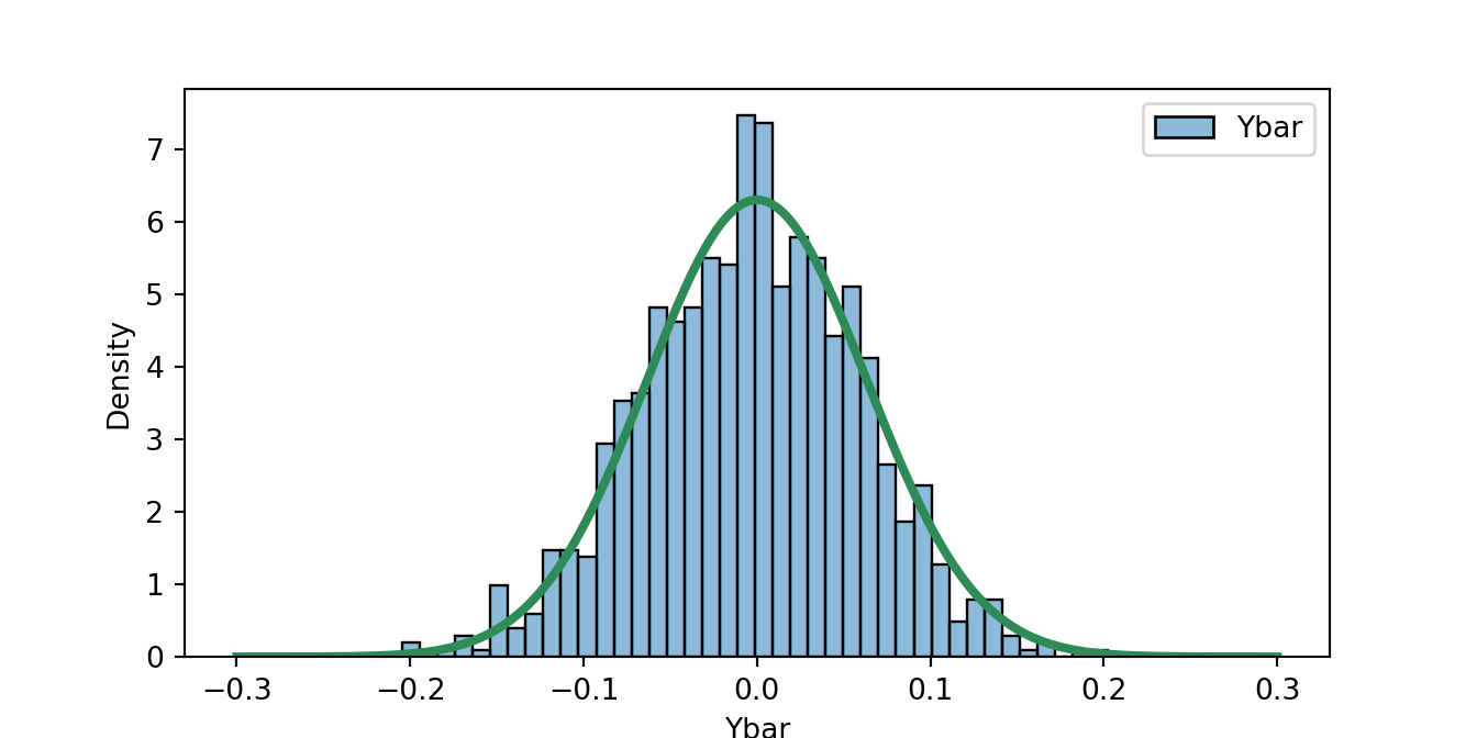
References
The Table is obtained from this Wikipedia page. Accessed on January 16, 2024.↩︎
The closing price adjusted for stock splits and dividends.↩︎
Typically the aggregation is done by averaging the observations at the high-frequency (e.g., daily) within each period of the lower frequency (e.g., monthly). Compactly, this can be done in a line of code:↩︎
You will need to create an API key in the FRED website at this link↩︎