6 High-Frequency Data
Since the 1990s the availability of intra-day transaction and quote data has sparkled research on existing questions and new ones have emerged from the analysis of the micro-structure of these markets. One of the old questions in financial econometrics is how to model and predict volatility as we discussed in the previous Chapter using several GARCH-type models. As we mentioned earlier, there has been a fair amount of research on realized volatility measures which represent an observable quantity for volatility based on intra-day returns. This approach is not only interesting because it provided an observable measure of volatility, but also because it contributed to the development of a new set of models that takes this measure as the dependent variable and try to explain it with time series and multivariate models. The scope of this Chapter is not so much to overview all of the interesting issues that arise with high-frequency data, but rather to get students started with the analysis of these data and constructing measures of realized volatility in R. To this goal, we will use the highfrequency package which provides several useful functions for data handling and construction of realized volatility measures.
The two main financial markets that provide high-frequency data are the FOREX and the US equity markets. The latter is contained in the TAQ (Trade And Quote) database which contains all trades (including quantity traded) and quotes for all listed stocks since the early 1990s. Contrary to this centralized market, the FOREX market is decentralized and there are only observations for quote of many currency pairs but no transaction data. An interesting issue of the FOREX market is that it is always open and geographically disperse since the trading day starts in Tokyo, which is followed by the opening of the London market, and finally by New York. In this Chapter we will consider exchange rates high-frequency data from TrueFX, a data provider which allows free access to high-frequency quote data from many years upon registration.
One big hurdle that we will encounter in this Chapter is that financial markets produce lots of data which require better data-handling tools and more computer power that has been needed so far. So, when you load the dataset, hold your breath and hope that your computer doesn’t crash!
6.1 Data management
Register for free to TrueFX and you will be able to download high-frequency data for a wide set of currencies. Due to the large amount of quotes, the data are provided in monthly files. For example, to load R the file for December 2013 of the USD/JPY (U.S. Dollar vs Japanese Yen) with the command data <- read.csv('USDJPY-2013-12.csv', header=FALSE) which took 14 seconds on a Intel Core i5 2.6 GHz and 8GB of RAM machine. Let’s first have a look at the data:
       V1                    V2      V3      V4
1 USD/JPY 20131202 00:00:00.320 102.488 102.495
2 USD/JPY 20131202 00:00:03.172 102.489 102.496
3 USD/JPY 20131202 00:00:03.732 102.490 102.496
4 USD/JPY 20131202 00:00:04.413 102.490 102.497
5 USD/JPY 20131202 00:00:09.104 102.490 102.497
The first column V1 represents the currency pair, the second column provides the date and time of the quote, and the third and forth columns represent the bid and ask quotes. The file consists of a total of 2276644 quotes that were produced in that month. Before starting to work on the data, we need to define the dataset as a time series object and it is thus important that we undestand the time format of the data provider and how to implement it in R. The first observation of the file is dated 20131202 00:00:00.320, that provides the day of the quote in the format YYYYMMDD followed by the time of the day in the format hh:mm:ss, with the seconds going from 00.000 to 61.000 that includes three decimals. The need to fraction the seconds is due to the high speed at which quotes and trades are produced in financial markets. So, the next step is to define the object data as a time series which requires to convert the second column of the file using the following command datetime <- strptime(data[,2], format="%Y%m%d %H:%M:%OS") which produces the following object:
[1] "2013-12-02 00:00:00.320 EST" "2013-12-02 00:00:03.172 EST" "2013-12-02 00:00:03.732 EST"
[4] "2013-12-02 00:00:04.413 EST" "2013-12-02 00:00:09.104 EST" "2013-12-02 00:00:15.895 EST"
We are now ready to define the file as a time series object in R and we are going to use the xts package which is particularly suitable to handle time and dates for high-frequency data. We discard the first and second columns, and just focus on the bid/ask quotes as shown below:
library(xts)
rate <- as.xts(data[,3:4], order.by=datetime)
colnames(rate) <- c("bid","ask")
head(rate)
bid ask
2013-12-02 00:00:00.319 102.488 102.495
2013-12-02 00:00:03.171 102.489 102.496
2013-12-02 00:00:03.732 102.490 102.496
2013-12-02 00:00:04.413 102.490 102.497
2013-12-02 00:00:09.104 102.490 102.497
2013-12-02 00:00:15.894 102.491 102.4976.2 Aggregating frequency
We have now created the xts object rate which contains the bid and ask quotes for the USD/JPY exchange rate in the month of December 2013. One of the first tasks in analyzing high-frequency data is to sub-sample the quotes at higher frequencies, such as 30 seconds, 1 or 5 minutes. One reason for sub-sampling is that at the second and micro-second level the quote and price changes are very small and contaminated by market microstructre noise, that is, erratic movements due to behavior of market participants interacting in the market rather than, for example, informational issues. A practical benefit of subsampling is that we discard many of the 2276644 observations and are able to work with smaller datasets which are easier to plot and analyze.
As an example, let’s say that we want to sub-sample the dataset at the 1 minute frequency. We achieve this by dividing the trading day in intervals of 1 minute and then pick the trade or quote that are closer in time to the 1 minute interval. The highfrequency package provides several functions to manage and analyze high-frequency data. The function aggregatets() has the purpose of aggregating the high-frequency quotes and trades to the desired frequency in seconds or minutes. In the example below, we sub-sample the mid-point between bid and ask USD/JPY exchange rate to the 1 minute frequency:
library(highfrequency)

midrate        <- (rate[,1]+rate[,2])/2
names(midrate) <- "midpoint"

midrate1m      <- aggregatets(midrate, on="minutes", k=1)
head(midrate1m)
midpoint
2013-12-02 00:01:00 102.525
2013-12-02 00:02:00 102.497
2013-12-02 00:03:00 102.505
2013-12-02 00:04:00 102.495
2013-12-02 00:05:00 102.495
2013-12-02 00:06:00 102.493The first observation corresponds to the last quote before 0, 1, 0, 2, 11, 113, 1, 335, 0, EST, -18000 as we can verify from analyzing the full dataset in the neighborhood of the first minute and all other quotes are discarded:
midpoint
2013-12-02 00:00:55.415 102.525
2013-12-02 00:00:55.592 102.525
2013-12-02 00:01:01.940 102.525
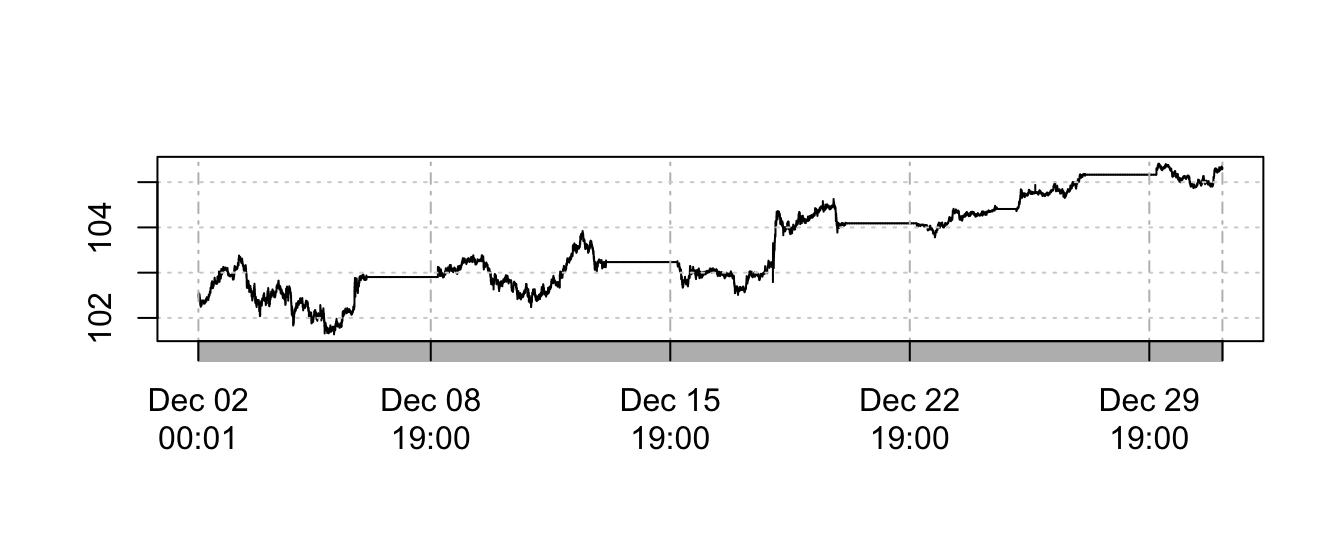
2013-12-02 00:01:06.908 102.526The result of the aggregation is a significant reduction of the sample size from 2276644 to 43096. We can now plot the time series of the exchange rate in December 2013 and the graph is shown below. It appears that there are periods in which the exchange rate is constant, which corresponds to weekends in which there is not much activity.
Since there is no price dynamics during weekends, we could decide to eliminate them from the sample and this can be achieved by eliminating the observations during the weekend as in the code below:
index <- .indexwday(midrate1m)
unique(index)
[1] 1 2 3 4 5 6 0# keep only Monday to Friday (day 1 to 5)
midrate1m <- midrate1m[index %in% 1:5]
plot(midrate1m, main="", type="p", pch=1, cex=0.05)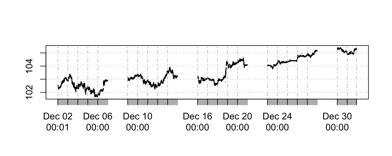
The plot looks similar to the earlier one because the line plot connects the By eliminating the week-ends the time series has reduced from 43096 to 31576.
The next thing is to calculate the returns that represent the percentage changes of the exchange rate at the 1 minute frequency. Below we calculate the returns and some summary statistics:
ret1m <- 100 * diff(log(midrate1m))
summary(ret1m)
Index midpoint
Min. :2013-12-02 00:01:00.00 Min. :-0.385477
1st Qu.:2013-12-09 11:34:45.00 1st Qu.:-0.005270
Median :2013-12-16 23:08:30.00 Median : 0.000000
Mean :2013-12-16 09:41:51.10 Mean : 0.000085
3rd Qu.:2013-12-24 10:42:15.00 3rd Qu.: 0.005359
Max. :2013-12-31 22:16:00.00 Max. : 0.491053
NA's :1 The mean and median are very close to zero with a minimum return of -0.385477% and maximum of 0.491053%. The standard deviation is 0.013521% which is expressed in terms of the 1-minute return.
6.3 Realized Volatility
One of the important applications of high-frequency data is to calculate non-parametric measures of volatility which are alternative to the GARCH modeling approach. These measures are then used to build a model to explain the volatility dynamics as well as for forecasting volatility. The simplest measure of realized volatility in day \(t\) is given by the sum of the square intra-day returns at frequency \(m\) (for a total of \(M\) returns in day \(t\)). In formula:
\[ RV_t = \sum_{m=1}^M R_{t,m}^2 \]
where \(R_{t,m}\) represents the \(m\)-th interval at a certain frequency of day \(t\). This can be implemented quite easily in R by selecting the intra-day return of each day, squaring them, and summing them up to produce the volatility measure in that day. However, we can avoid the programming effort since the highfrequency package provides functions to calculate the realized volatility measure at the chosen frequency. The rCov() function allows to calculate the realized volatility for the specificied return time series and at the appropriate frequency:
rv1m   <- rCov(ret1m, align.by="minutes", align.period=1)
plot(rv1m^0.5, ylim=c(0, 1.1*max(rv1m^0.5)), main="", type="b")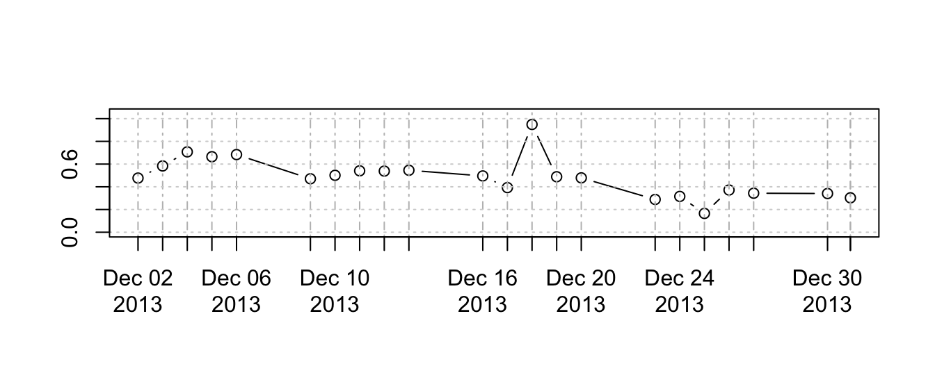
The plot shows the time series of realized volatility for the daily return of the USD/JPY in December 2013 obtained from the 1 minute returns. An important choice that has to be made concerns the time interval to use for the intra-day returns. Ideally, we would like to calculate returns over short intervals which would allow to increase the sample size of square returns of each day that the realized volatility is calculated. On the other hand, very high-frequency returns introduce microstructure noise that might bias the volatility measure and increase the variability of the volatility measure. In the example below, we compare realized volatility measures from returns at the 10 seconds, 1 minute, and 10 minutes frequency. The results show that the measure obtained from the 10-seconds return overall tracks the measures obtained with the higher frequencies, except for December 26th, 2013, when the volatility calculated on the 10-sec returns spikes up to almost 1% whilst the other two measures stay below 0.4% on that day. Overall, there is no optimal way to choose the interval to use, but for a wide class of assets many researchers have converged on using the 5-minute frequency to calculate realized volatility measures.
rv10s       <- rCov(ret10s, align.by="seconds", align.period=10)
rv10m       <- rCov(ret10m, align.by="minutes", align.period=10)
plot(rv10s^0.5, ylim=c(0, maxy), main="", lty=1)  # black continuous
lines(rv1m^0.5,  col=2, lty=2, lwd=2)             # red dashed
lines(rv10m^0.5, col=3, lty=3, lwd=2)             # green dots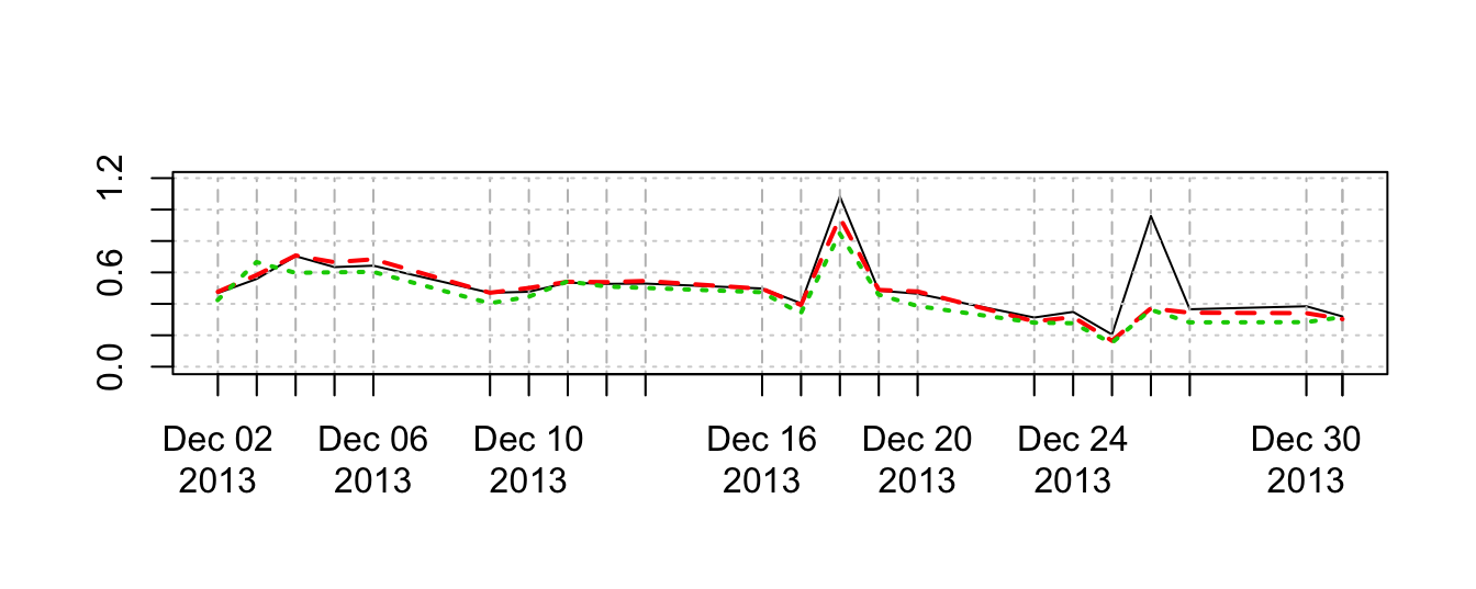
The realized volatility measure \(RV_t\) is criticized because it is not robust to microstructure noise and to outliers of jumps, as it is shown in the previous graph. An alternative to the \(RV_t\) estimator is the median RV estimator which consists of the taking the median of the intra-day returns
medrv5m  <- medRV(ret5m, align.by="minutes", align.period=5)
plot(medrv5m^0.5, ylim=c(0,maxy), main="",lty=1)
lines(rv5m^0.5, col=2, lty=2, lwd=2)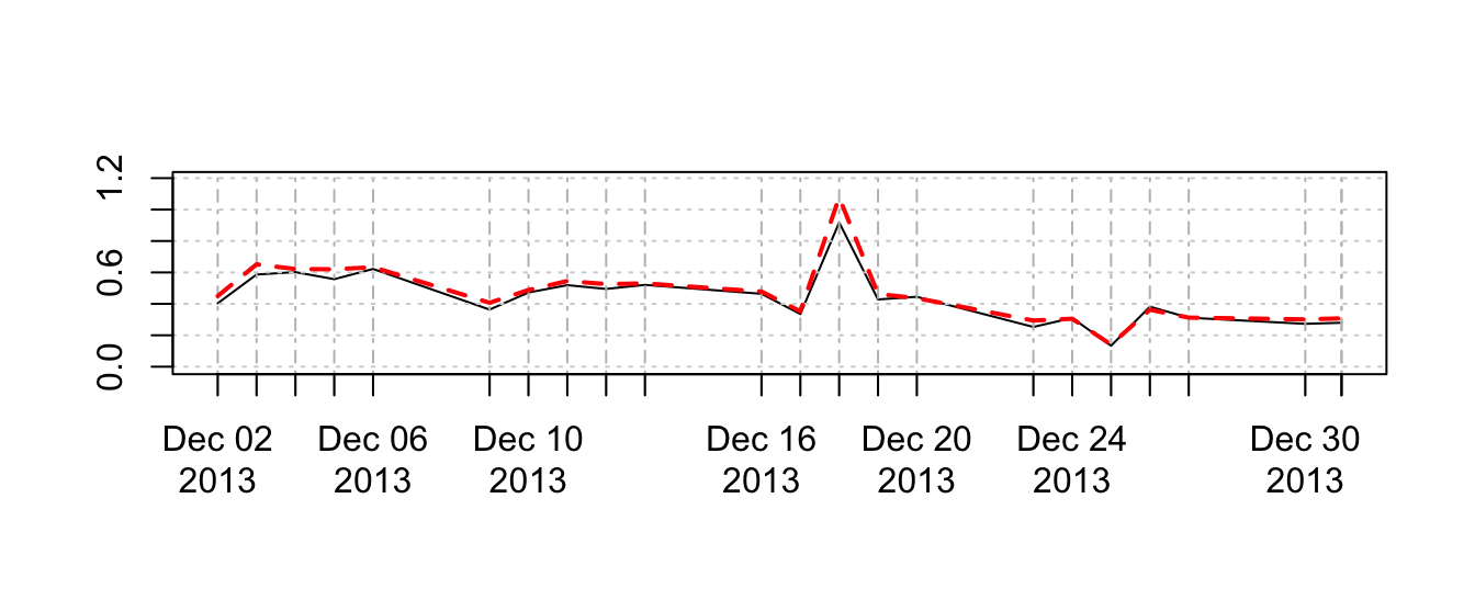
6.4 Modeling realized volatility
AR(1) model for realized volatility: \[ RV_t = \beta_0 + \beta_1 * RV_{t-1} + \epsilon_t \]
Heterogeneous AR HAR(1) for realized volatlity: \[ RV_t = \beta_0 + \beta_1 * RV_{t-1} + \beta_2 * \hat{RV}^5_{t-1} + \beta_3 * \hat{RV}^{22}_{t-1} + \epsilon_t \] where the 5 and 22 day moving averages are defined as \(\hat{RV}^5_{t-1} = \sum_{j=1}^5 R_{t-j} /5\) and \(\hat{RV}^{22}_{t-1} = \sum_{j=1}^{22} R_{t-j} /22\).
To be completed.