5 Volatility Models
A stylized fact across many asset classes is that the standard deviation of returns, also referred to as volatility, varies significantly over time. Figure 5.1 shows the time series of the daily percentage returns of the S&P 500 and of the Japanese Yen to US Dollar exchange rate from January 1980 until May 2017. The horizontal dashed lines represent a 95% confidence interval obtained as the sample average return plus/minus 1.96 times the sample standard deviation of the returns. A features that emerges from the Figure is that financial returns stay within these bands for long periods of time followed by periods of large positive and negative returns that last for several months or years. Hence, the dispersion of the distribution of returns in any given day seems to be different with some periods of high volatility and others prolonged periods of low volatility. So far we have discussed models for the expected return, that is \(E(R_{t+1})\), but now we are arguing that we should also consider models for the expected variance of returns, \(Var(R_{t+1})\). Modeling volatility is thus a important area of financial econometrics since it provides a measure of risk which is an important input to many financial decisions (e.g., from option pricing to risk management).
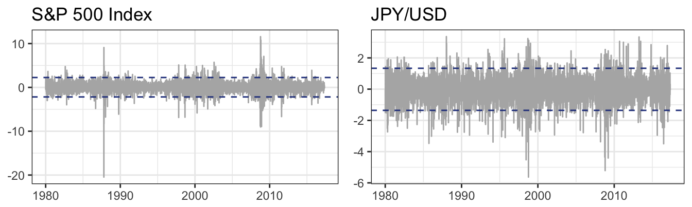
Figure 5.1: Daily percentage returns of the SP 500 Index and the Japanese Yen to US Dollar exchange rates starting in January 1980.
A measure of market volatility exist already and is represented by the CBOE Volatility Index (or VIX). The VIX is obtained from the implied volatilities of S&P 500 Index option prices and it is interpreted as a measure of market risk or uncertainty contained in option prices. Figure 5.2 shows the daily time series of the VIX since January 1990 on an annualized scale. Although a measure of volatility such as VIX is available for the S&P 500, for many other assets such a measure is not available and we can either construct it based on option prices or based on historical returns.
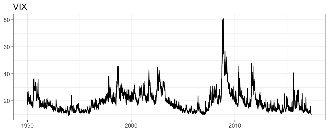
Figure 5.2: The CBOE Volatility Index (VIX) at the daily frequency since January 1990.
This Chapter discusses several approaches that can be used to model and forecast volatility based on historical returns. The basic setup that we consider is a model that assumes that returns at time \(t+1\), denoted \(R_{t+1}\), are defined as: \[R_{t+1} = \mu_{t+1} + \eta_{t+1}\] This model decomposes the return \(R_{t+1}\) in two components:
- Expected return: \(\mu_{t+1}\) represents the predictable part or the expected return of the asset. At the daily and intra-daily frequency, this component is typically assumed equal to zero. Alternatively, it could be assumed to follow an AR(p) process \(\mu_{t+1} = \phi_0 + \phi_1 * R_{t} + \cdots + \phi_p * R_{t-p+1}\) or being a function of other contemporaneous or lagged variables, that is, \(\mu_{t+1} = \phi_0 + \phi_1 * X_t + \phi_2 X_{t-1}\).
- Shock: \(\eta_{t+1}\) is the unpredictable component of the return; it can assumed to be equal to \(\eta_{t+1} = \sigma_{t+1}\epsilon_{t+1}\) where:
- Volatility: \(\sigma_{t+1}\) is the standard deviation of the shock conditional on information available at time \(t\); in a time series model volatility is a function of past returns, e.g., \(\sigma^2_{t+1} = \omega + \alpha R_t\).
- Standardized shock: \(\epsilon_{t+1}\) represents the shock which is assumed to have mean 0 and variance 1. A typical assumption is that it is normally distributed, but alternative distributional assumption can be introduced such as a \(t\) distribution that allows for fatter tails.
The aim of this Chapter is to discuss different models to estimate and forecast \(\sigma_{t+1}\) using simple techniques such as Moving Average (MA) and Exponential Moving Average (EMA), followed by a discussion of a time series model such as the Auto-Regressive Conditional Heteroskedasticy (ARCH) model. ARCH models have been extended in several directions, but for the purpose of this Chapter we will consider the two most important generalizations: GARCH (Generalized ARCH) and GJR-GARCH (Glosten, Jagganathan and Runkle ARCH) that includes an asymmetric relationship between the shocks and the conditional variance.
5.1 Moving Average (MA) and Exponential Moving Average (EMA)
A simple approach to estimate the conditional variance is to average the square returns over a recent window of observations, for example the last \(M\) observations. The Moving Average (MA) estimate of the variance in day \(t\), \(\sigma^2_{t+1}\), is given by \[ \sigma^2_{t+1} = \frac{1}{M}\left(R_{t}^2 + R^2_{t-1}+ \cdots + R^2_{t-M+1}\right) = \frac{1}{M}\sum_{j=1}^{M} R^2_{t-j+1}\] and the standard deviation is calculated as \(\sqrt{\sigma^2_{t+1}}\). The two extreme values of the window are \(M=1\), which implies \(\sigma^2_{t+1} = R_{t}^2\), and \(M=t\), that leads to \(\sigma^2_{t+1} = \sigma^2\), where \(\sigma^2\) represents the unconditional variance estimated on the full sample. Small values of \(M\) imply that the volatility estimate is very responsive to the most recent square returns, whilst for large values of \(M\) the estimate responds very little to the latest returns. Another way to look at the role of the window size on the smoothness of the volatility is to interpret it as an average of the last \(M\) days each carrying a weight of \(100/M\)% (i.e., for \(M=25\) the weight is 4%). When \(M\) increases, the weight given to each observation in the window becomes smaller so that each daily square return (even when extreme) has a smaller impact on changing the volatility estimate. The discussion so far represents the typical implementation of the MA approach which relies on the assumption that \(\mu_{t+1} = 0\) so that \(R_{t+1} = \eta_{t+1}\). More generally, we might want to include an intercept or assume that the expected return follows a AR(1). In this case, the MA is calculated by averaging the squares of \(\eta_{t+1}\) calculated as \(\eta_{t+1} = R_{t+1} - \mu_{t+1}\).
The MA approach can be implemented in R using the rollmean() function provided in package zoo which requires to specify the window size (\(M\) in the notation above). An example for the S&P 500 daily returns is provided in Figure 5.3:
GSPC              <- getSymbols("^GSPC", from="1980-01-01", auto.assign=FALSE)
sp500daily        <- 100 * ClCl(GSPC) %>% na.omit
names(sp500daily) <- "RET"
sigma25           <- zoo::rollmean(sp500daily^2, 25, align="right")
names(sigma25)    <- "MA25"
ggplot(merge(sigma25, sp500daily)) + geom_line(aes(time(sp500daily), abs(RET)),color="gray80") +
  theme_bw() + geom_line(aes(index(sp500daily), MA25^0.5), color="orangered3")  +
  labs(x=NULL, y=NULL)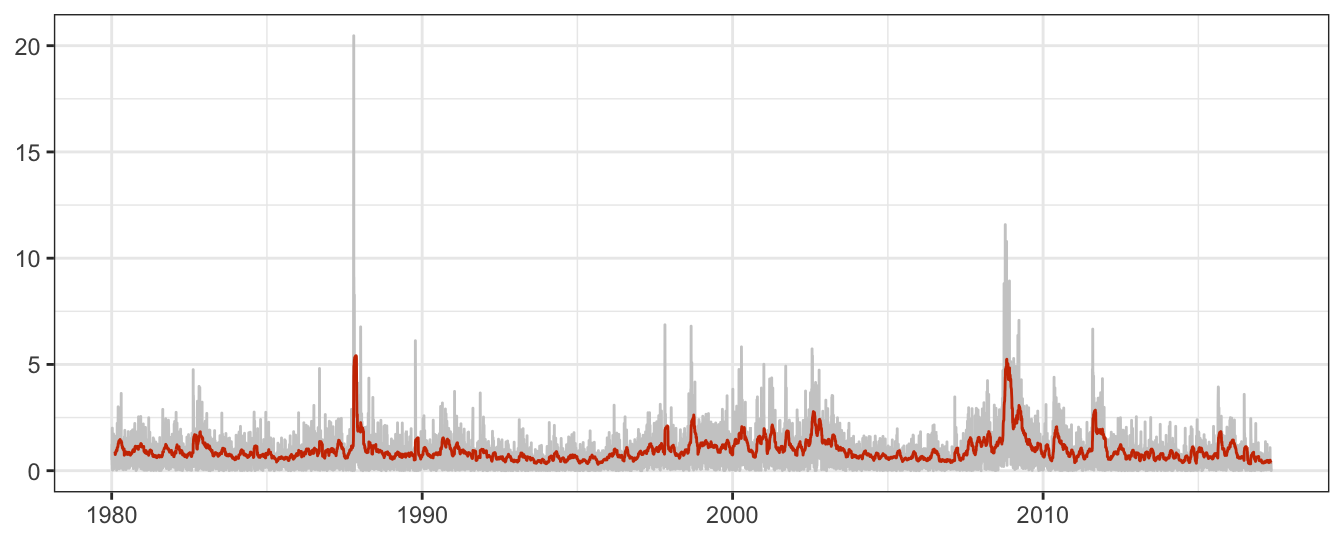
Figure 5.3: Absolute returns of the SP 500 Index and the Moving Average (MA) with parameter M set to 25.
The effect of increasing the window size from \(M=25\) (continuous line) to \(100\) (dashed line) is shown in Figure 5.4: the longer window smooths out the fluctuation of the MA(25) since each observation is given a smaller weight. This implies that large (negative or positive) returns increase volatility less when using longer windows relative to shorter ones.
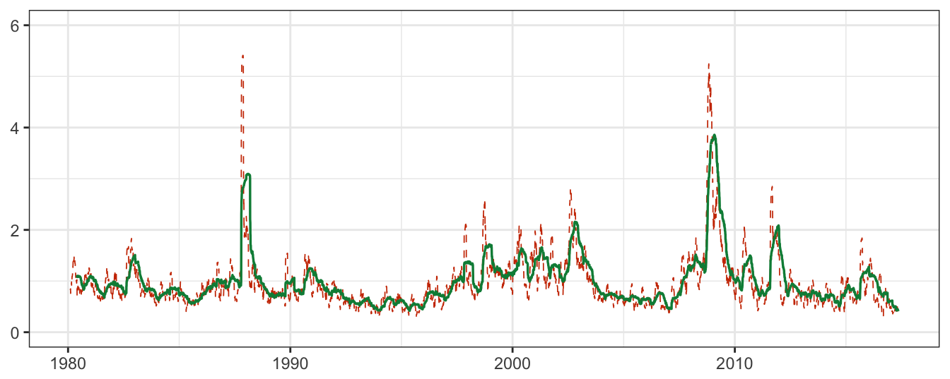
Figure 5.4: The Moving Average (MA) with parameter M set to 25 and 100. Can you guess if the dashed line corresponds to M equal to 25 or 100 days?
One drawback of the MA approach is that large daily returns are able to increase/decrease significantly the volatility estimate when they enter/exit the window of \(M\) days. An extension of the MA approach is to have a smoothly decreasing weight assigned to older returns instead of the discrete jump of the weight from \(1/M\) to 0 at the \(M+1\)th observation. This approach is called Exponential Moving Average (EMA) and gained popularity in finance since the investment bank J.P. Morgan proposed it as a model to predict volatility for Value-at-Risk (VaR) calculations. The EMA with parameter \(\lambda\) is calculated as follows:
\[ \sigma^2_{t+1} = \lambda \sum_{j=1}^{\infty} (1-\lambda)^{j-1} R^2_{t-j+1} \] where \(\lambda\) is a smoothing parameter between zero and one. After some algebra, the expression above can be rewritten as follows:
\[ \sigma^2_{t+1} = (1-\lambda) * \sigma^2_{t} + \lambda R^2_t \]
which shows that the conditional variance estimate in day \(t+1\) is given by a weighted average of the previous day estimate and the square return in day \(t\), with the weights equal to \(1-\lambda\) and \(\lambda\), respectively. A typical value of \(\lambda\) is 0.06 which means that day \(t\) has a 6% weight in calculating the volatility forecast, day \(t-1\) has weight (0.94 * 6) = 5.64%, day \(t-2\) has weight (0.94\(^2\) * 6) = 5.3016%, day \(t-k\) has weight (0.94\(^k\) * 6)% and so on. Figure 5.5 shows the MA and EMA weight on past observations. The MA method assigns a positive and constant weight to the last \(M\) observations as opposed to the EMA approach that spreads the weight over a longer period and weights differently more recent observation relative to older ones.
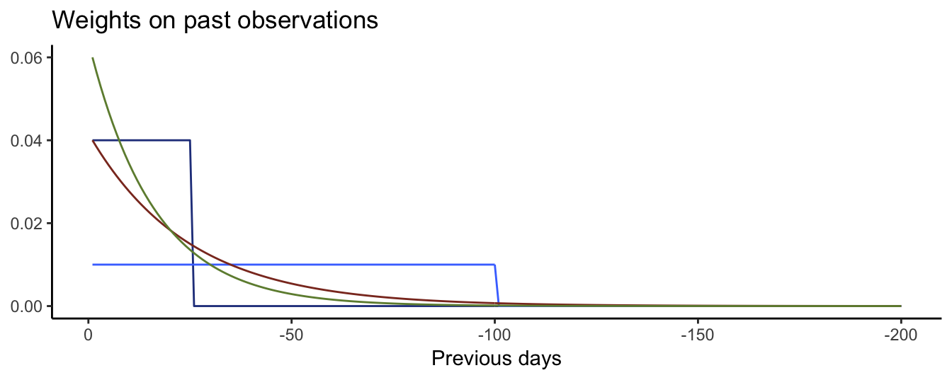
Figure 5.5: Weight on past values for MA with M equal to 25 and 100 and EMA equal to 0.04 and 0.06.
The typical value for \(M\) is 25 (one trading month) and for \(\lambda\) it is 0.06. The graph below compares the volatility estimates from the MA(25) and EMA(0.06) methods. In this example we use the package TTR that provides functions to calculate moving averages, both simple and of the exponential type:
library(TTR)
# SMA() function for Simple Moving Average; n = number of days
ma25  <- SMA(sp500daily^2, n=25)
names(ma25) <- "MA25"
# EMA() function for Exponential Moving Average; ratio = lambda
ema06 <- EMA(sp500daily^2, ratio=0.06)
names(ema06) <- "EMA06"
autoplot(merge(ma25, ema06)^0.5, ncol=2) + theme_bw()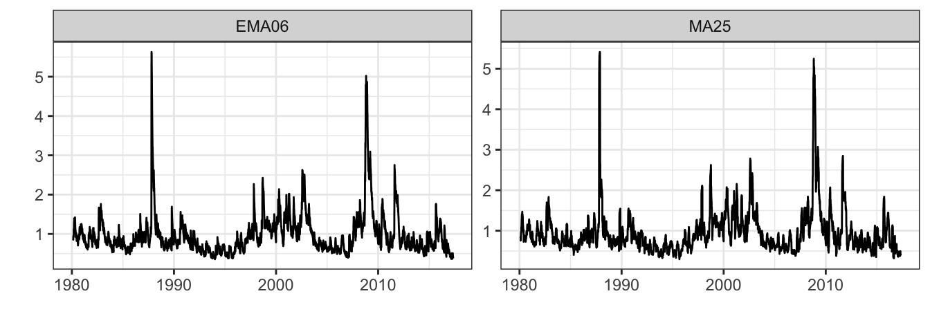
Figure 5.6: Time series of the MA(25) and EMA(0.06) volatility estimates.
Figure 5.6 shows the MA and EMA daily volatility estimate for over 23 years and, at this scale, it is difficult to see large differences between the two methods. However, by plotting a sub-period of time, some differences become evident. Figure 5.7 shows the period between beginning 2008 and end of 2009. The biggest difference between the two methods is that in periods of rapid change (from small/large to large/small absolute returns) the EMA line captures the change in volatility regime more smoothly relative to the simple MA. This is in particular clear in the second part of 2008 and the beginning of 2009, with some differences between the two lines.
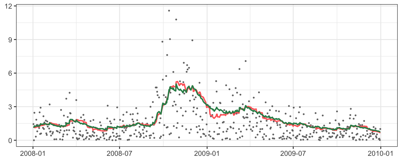
Figure 5.7: Volatility estimates of MA(25) and EMA(0.06) from January 2008 to December 2009. The dots represents the absolute daily returns.
The parameters of MA and EMA are, usually, chosen a priori rather than being estimated from the data.
There are possible ways to estimate these parameters although they are not popular in the financial literature and typically do not provide great benefit for practical purposes. In the following Section we discuss a more general volatility model which generalizes the EMA model and it is typically estimated from the data.
5.2 Auto-Regressive Conditional Heteroskedasticity (ARCH) models
The ARCH model was proposed by Engle (1982) to model the time-varying variance of the inflation rate. Since then it has gained popularity in finance as a way to model the changes in the volatility of asset returns. Assuming that \(\mu_{t+1} = 0\) as in the previous Sections, the model simplifies to \(R_{t+1} = \eta_{t+1} = \sigma_{t+1}\epsilon_{t+1}\), that is, the return next period is given by an exogenous shock, \(\epsilon_{t+1}\), amplified by the time-varying volatility, \(\sigma_{t+1}\)39. The conditional variance \(\sigma^2_{t+1}\) can be assumed to be a function of the previous period square return, that is, \[\sigma^2_{t+1} = \omega + \alpha * R_{t}^2\] where \(\omega\) and \(\alpha\) are parameters to be estimated. The AR part in the ARCH name relates to the fact that the variance of returns is a function of the lagged (square) returns. This specification is called the ARCH(1) model and can be generalized to include \(p\) lags which results in the ARCH(p) model: \[\sigma^2_{t+1} = \omega + \alpha_1 * R_{t}^2 + \cdots + \alpha_p * R_{t-p+1}^2\] The empirical evidence indicates that financial returns typically require \(p\) to be large. A parsimonious alternative to the ARCH model is the Generalized ARCH (GARCH) model which is characterized by the following Equation for the conditional variance: \[\sigma^2_{t+1} = \omega + \alpha * R_{t}^2 + \beta * \sigma^2_{t}\] In this case the variance is affected by \(R_t^2\) as well as by last period conditional variance \(\sigma_t^2\). This specification is parsimonious, relative to an ARCH model with large \(p\), since all past square returns are included in \(\sigma^2_{t-1}\), but using only 3 parameters rather than of \(p+1\). The specification above represents a GARCH(1,1) model since it includes one lag of the square return and the conditional variance. However, it can be easily generalized to the GARCH(p,q) case in which \(p\) lags of the square return and \(q\) lags of the conditional variance are included. The empirical evidence suggests that the GARCH(1,1) is typically the best model for several asset classes and it is only in rare instances outperformed by \(p\) and \(q\) different from 1.
We can derive the mean of the conditional variance in the case of the GARCH(1,1) which is given by: \[ \sigma^2 = \omega / (1-(\alpha + \beta))\] where \(\sigma^2 = E(\sigma^2_{t+1})\) and represents the unconditional variance as opposed to \(\sigma^2_t\) that denotes the conditional variance of the returns. The difference between these quantities is that \(\sigma^2_{t+1}\) is a forecast of volatility based on the information available at time \(t\), while \(\sigma^2\) represents the time-average of the conditional forecasts. The Equation for \(\sigma^2\) indicates that a condition for the variance to be finite is that \(\alpha + \beta < 1\). If this condition is not satisfied, the variance of the returns is infinite and volatility behaves like a random walk model, rather than being mean-reverting. This situation is similar to the case of the AR(1) in which a coefficient (in absolute value) less than 1 ensures that the time series is stationary, and thus mean-reverting. We can think similarly about the case of the variance, where the condition that \(\alpha+\beta < 1\) guarantees that volatility is stationary and mean reverting. What does it mean that variance (or volatility) is mean reverting? It means that volatility might be highly persistent, but oscillates between periods in which it is higher and lower than its unconditional level \(\sigma\). This interpretation is consistent with the empirical observation that volatility switches between periods in which it is high and others in which it is low. On the other hand, non-stationary volatility implies that periods of high volatility (i.e., higher than average) are expected to persist in the long run rather than reverting back to the unconditional variance. The same holds for periods of low volatility which, in case of non-stationarity, is expected to last in the long run. This distinction is practically relevant, in particular when the interest is to forecast future volatility and at long horizons.
The distinction between mean-reverting (i.e., stationary) and non-stationary volatility is an important property that differentiates volatility models. In particular, the EMA model can be considered a special case of the GARCH model when the parameters are set equal to \(\omega = 0\), \(\alpha = \lambda\) and \(\beta = 1-\lambda\). This shows that EMA imposes the assumption that \(\alpha + \beta = 1\), and thus that volatility is non-stationary. Empirically, this hypothesis can be tested by assuming the null hypothesis \(\alpha+ \beta = 1\) versus the one sided hypothesis that \(\alpha + \beta < 1\).
Another popular GARCH specification was proposed by Glosten, Jagganathan and Runkle (hence, GJR-GARCH) which assumes that the square return has a different effect on volatility depending on its sign. The conditional variance Equation of this model is:
\[\sigma^2_{t+1} = \omega + \alpha_1 * R_{t}^2 + \gamma_1 R_{t}^2 * I(R_{t} \leq 0) + \beta * \sigma^2_{t}\]
In this specification, when the return is positive its effect on the conditional variance is \(\alpha_1\) and when it is negative the effect is \(\alpha_1 + \gamma_1\). Testing the hypothesis that \(\gamma_1 = 0\) thus provides a test of the symmetry of the effect of shocks on volatility. The estimation of the model on asset returns from many asset classes shows that \(\alpha_1\) is estimated close to zero and insignificant, while \(\gamma_1\) is found positive and significant. The evidence thus suggests that negative shocks lead to more uncertainty and an increase in the volatility of asset returns, while positive shocks do not have a relevant effect.
5.2.1 Estimation of GARCH models
ARCH/GARCH models cannot be estimated using OLS because the model is nonlinear in parameters40 The estimation of GARCH models is thus performed using an alternative estimation technique called Maximum Likelihoood (ML). The ML estimation method represents a general estimation principle that can be applied to a large set of models, not only to volatility models.
It might be useful to first discuss the ML approach to estimation in comparison to the familiar OLS approach. The OLS approach is to choose the parameter values that minimize the sum of the square residuals which measures the unfitness of the model to explain the data for a certain set of parameter values. Instead, the approach of ML is to choose the parameter values that maximize the likelihood or probability that the data were generated by the model. For the case of a simple AR model with homoskedastic errors it can be shown that the OLS and ML estimators are equivalent. A difference between OLS and ML is that the first provides analytical formula for the estimation of linear models, whilst the ML estimator is the result of numerical optimization.
We assume that volatility models are of the general form discussed earlier, i.e., \(R_{t+1} = \mu_{t+1} + \sigma_{t+1}\epsilon_t\). Based on the distributional assumption introduced earlier, we can say that the standardized residuals \((R_{t+1} - \mu_{t+1})/\sigma_{t+1}\) should be normally distributed with mean 0 and variance 1. Bear in mind that both \(\mu_{t+1}\) and \(\sigma^2_t\) depend on parameters that are denoted by \(\theta_\mu\) and \(\theta_\sigma\). For example, for an AR(1)-GARCH(1,1) model the parameter of the mean is \(\theta_\mu = (\phi_0, \phi_1)\) and the parameters of the conditional variance is \(\theta_\sigma = (\omega, \alpha, \beta)'\). Given the assumption of normality, the density or likelihood function of \(R_{t+1}\) is \[ f(R_{t+1} | \theta_\mu, \theta_\sigma) = \frac{1}{\sqrt{2 \pi \sigma^2_{t+1}(\theta_\sigma)}} \exp\left[ - \frac{1}{2}\left(\frac{R_{t+1} - \mu_{t+1}(\theta_\mu)}{\sigma_{t+1}(\theta_\sigma)}\right)^2\right] \] which represents the normal density for the return in day \(t+1\). We wrote the conditional mean and variance as \(\mu_{t+1}(\theta_\mu)\) and \(\sigma^2_t(\theta_\sigma)\) to make explicit their dependence on parameters over which the likelihood function will be maximized. Since we have \(T\) returns, we are interested in the joint likelihood of the observed returns and denoting by \(p\) the largest lag of \(R_{t+1}\) used in the conditional mean and variance, we can define the (conditional) likelihood function \(\mathcal{L}(\theta_\mu, \theta_\sigma)\) (\(=f(R_{p+1}, \cdots, R_{t+1} | \theta_\mu, \theta_\sigma, R_1, \cdots, R_{p})\)) as \[ \mathcal{L}(\theta_\mu, \theta_\sigma) = \prod_{t=p+1}^T f(R_{t+1} | \theta_\mu, \theta_\sigma) = \prod_{t=p+1}^T \frac{1}{\sqrt{2 \pi\sigma^2_{t+1}(\theta_\sigma)}} \exp\left[ - \frac{1}{2}\left(\frac{R_{t+1} - \mu_{t+1}(\theta_\mu)}{\sigma_{t+1}(\theta_\sigma)}\right)^2\right] \] The ML estimates \(\hat\theta_\mu\) and \(\hat\theta_\sigma\) are thus obtained by maximizing the likelihood function \(\mathcal{L}(\theta_\mu, \theta_\sigma)\). It is convenient to log-transform the likelihood function to simplify the task of maximizing the function. We denote the log-likelihood by \(l(\theta_\mu, \theta_\sigma)\) and it is given by \[ l(\theta_\mu, \theta_\sigma) = \ln \mathcal{L}(\theta_\mu, \theta_\sigma) = -\frac{1}{2} \sum_{t=p+1}^T \left[ \ln(2\pi) + \ln \sigma^2_{t+1}(\theta_\sigma) +\left(\frac{R_{t+1} - \mu_{t+1}(\theta_\mu)}{\sigma_{t+1}(\theta_\sigma)} \right)^2 \right] \] since the first term \(\ln(2\pi)\) does not depend on any parameter, it can be dropped from the function. The estimates \(\hat\theta_\mu\) and \(\hat\theta_\sigma\) are then obtained by maximizing \[ l(\theta_\mu, \theta_\sigma) = -\frac{1}{2} \sum_{t=p+1}^T \left[ \ln \sigma^2_{t+1}(\theta_\sigma) +\left(\frac{R_{t+1} - \mu_{t+1}(\theta_\mu)}{\sigma_{t+1}(\theta_\sigma)}\right)^2 \right] \] The maximization of the likelihood or log-likelihood is performed numerically, which means that we use algorithms to find the maximum of this function. The problem with this approach is that, in some situations, the likelihood function is not well-behaved and characterized by local maxima. The numerical search has to be started at some initial values and, in the difficult cases just mentioned, the choice of these values is extremely important to achieve the global maximum of the function. The choice of valid starting values for the parameters can be achieved by a small-scale grid search over the space of possible values of the parameters.
In the case of volatility models the likelihood function is usually well-behaved and achieves a maximum quite rapidly. In the following Section we discuss some R packages that implement GARCH estimation and forecasting.
5.2.2 Inference for GARCH models
… coming soon (or later) …
5.2.3 GARCH in R
There are several packages that provide functions to estimate models from the GARCH family. One of the earliest is the garch() function in the tseries package, which is however quite limited in the type of models it can estimate. More flexible functions for GARCH estimation are provided by the package fGarch, that allows to specify the conditional mean \(\mu_{t+1}\) and the conditional variance \(\sigma^2_{t+1}\). The function to perform the estimation is called garchFit. The example below shows the application of the garchFit function to the daily returns of the S&P 500 index. The first example estimates a GARCH(1,1) with only the intercept in the conditional mean (i.e., \(\mu_{t+1} = \mu\)) and then consider an AR(1) for the conditional mean (i.e., \(\mu_{t+1} = \mu + \beta_1 R_t\)) which we denote as the AR(1)-GARCH(1,1) model. Notice that to specify the AR(1) for the conditional mean we use the function arma(p,q) which is a more general function than those used to estimate AR(p) models.
library(fGarch)
fit <- garchFit(~garch(1,1), data=sp500daily, trace=FALSE)
round(fit@fit$matcoef, 3)
Estimate Std. Error t value Pr(>|t|)
mu 0.059 0.008 7.110 0
omega 0.015 0.002 7.116 0
alpha1 0.082 0.006 14.097 0
beta1 0.905 0.007 133.003 0The output provides standard errors for the parameter estimates as well as t-stats and p-values for the null hypothesis that the coefficients are equal to zero. The results show that the mean \(\mu\) is estimated equal to 0.059% and it is statistically significant even at 1%. Hence, for the daily S&P 500 returns the assumption of a zero expected return is rejected. The estimate of \(\alpha\) is 0.082 and of \(\beta\) is 0.905, with their sum equal to 0.987, which is quite close enough to 1 to conclude that volatility is very persistent and close to being non-stationary. It might also be interesting to evaluate the need to introduce some dependence in the conditional mean, for example, by assuming an AR(1) model. The command arma(1,0) + garch(1,1) in the garchFit() function estimates an AR(1) model with GARCH(1,1) conditional variance:
fit <- garchFit(~ arma(1,0) + garch(1,1), data=sp500daily, trace=FALSE)
round(fit@fit$matcoef, 3)
Estimate Std. Error t value Pr(>|t|)
mu 0.059 0.008 7.070 0.000
ar1 0.004 0.011 0.351 0.726
omega 0.016 0.002 7.117 0.000
alpha1 0.082 0.006 14.097 0.000
beta1 0.905 0.007 132.954 0.000The estimate of the AR(1) coefficient is 0.004 and it is not statistically significant at 10% level, which shows the irrelevance of including dependence in the conditional mean of daily financial returns.
Based on the GARCH model estimation, we can then obtain the conditional variance \(\hat{\sigma_t^2}\) and the conditional standard deviation \(\hat{\sigma_t}\). The conditional standard deviation is extracted by appending @sigma.t to the garchFit object:
sigma <- fit@sigma.t  # class is numeric
qplot(time(sp500daily), sigma, geom="line", xlab=NULL, ylab="") +
  theme_bw() + labs(title="Conditional standard deviation")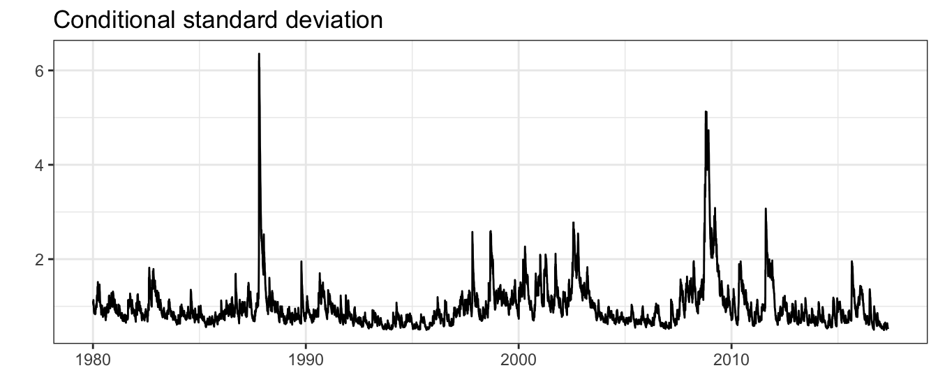
Figure 5.8: Conditional standard deviation estimated by the AR(1)-GARCH(1,1) model for the SP500 returns.
Figure 5.8 shows the significant variation over time of the standard deviation that alternates between periods of low and high volatility, in addition to sudden increases in volatility due to the occurrence of large returns. It is also interesting to compare the fitted standard deviation from the GARCH model with the ones obtained from the MA and EMA methods. The correlation between the MA and GARCH conditional standard deviation is 0.967 and between EMA and GARCH is 0.981 and, to a certain extent, they can be considered very good substitutes for each other (in particular at short horizons). Figure 5.9 shows the scatter plot of the conditional standard deviation for the GARCH model vs the MA and EMA estimates. Points above/below the diagonal represent days in which the GARCH estimate is larger/smaller relative to the MA/EMA estimates. The largest differences occur for the volatility estimates obtained with the MA method for values larger than 5%. This is due to the different reaction of \(\sigma^2_{t+1}\) to large (absolute) returns in the MA models relative to the GARCH and EMA models.
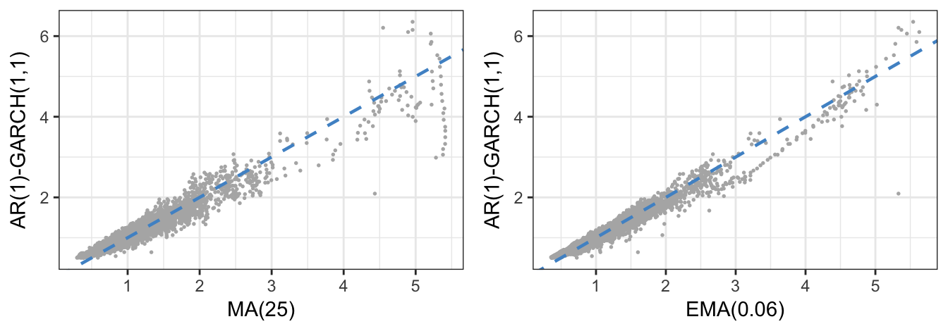
Figure 5.9: Comparison of the estimated standard deviation from the GARCH(1,1) model and from the EMA with parameter equal to 0.06.
The residuals of the GARCH model can also provide valuable information about the goodness of the model in explaining the returns. Appending @residuals to the garchFit estimation object we can extract the residuals of the GARCH model that represent an estimate of \(\sigma_{t+1}\epsilon_{t+1}\). Figure 5.10 shows that the residuals maintain most of the characteristics of the raw returns, in particular the clusters of volatility. This is because these residuals have been obtained from the last fitted model in which \(\hat\mu_{t+1} =\) 0.059 + (0.004) \(* R_{t-1}\) and the residuals are thus given by \(R_{t+1} - \hat\mu_{t+1}\). The contribution of the intercept is to demean the return series while the small coefficient on the lagged return leads to returns that are very close to the residuals.
res <- fit@residuals  # class is numeric
p1  <- qplot(time(sp500daily), res, geom="line", main="UNstandardized Residuals") +
  labs(x=NULL, y=NULL) + theme_bw()
p2  <- qplot(time(sp500daily), res/sigma, geom="line", main="Standardized Residuals") +
  labs(x=NULL, y=NULL) + theme_bw()
gridExtra::grid.arrange(p1, p2, ncol=2)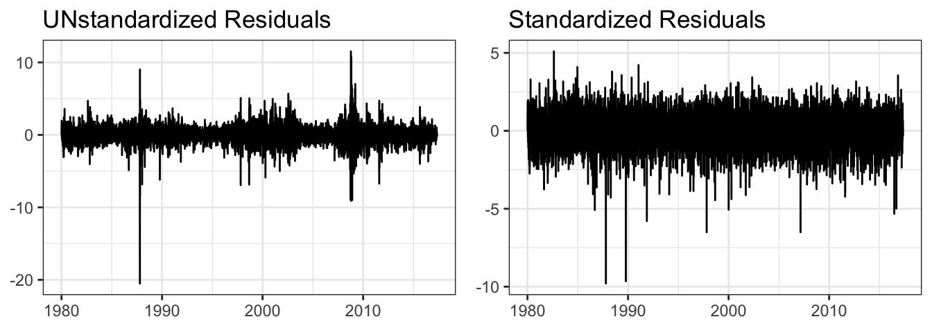
Figure 5.10: Standardized and unstandardized residuals for the SP500 daily returns using the AR(1)-GARCH(1,1) model.
Figure 5.10 shows the time series of the residuals \(\sigma_{t+1}\epsilon_{t+1}\) together with the standardized residuals \(\epsilon_{t+1}\) which should satisfy the properties of being independent over time (i.e., no auto-correlation) and normally distributed (given our earlier assumptions). The time series of the standardized residuals seem to be exempt from heteroskedasticity (e.g., volatility clustering) which has been taken into account by \(\sigma_{t+1}\). However, we notice a few large negative standardized residuals that are quite unlikely to happen assuming a normal distribution.
The first property of the standardized residuals is that they should be approximately normally distributed. To assess this assumption, Figure 5.11 compares the histogram of the standardized residuals with the standard normal distribution. The histogram of the standardized residuals has a large peak at the center of the distribution and fatter left tail relative to the normal, although this is difficult to see in the graph. However, calculating the skewness of the standardized residuals, equal to -0.455, and the excess kurtosis, equal to -0.455, indicate that the large negative returns in the time series plot point to the deviation of the standardized returns distribution from normality. We can conclude that the normality assumption we made earlier seems not to be supported in the data in favor of a distribution with fatter tails and possibly skewed. However, the skewness could also be due to misspecification of the conditional variance in the sense that the GARCH(1,1) model might be missing some important features of the volatility dynamics.
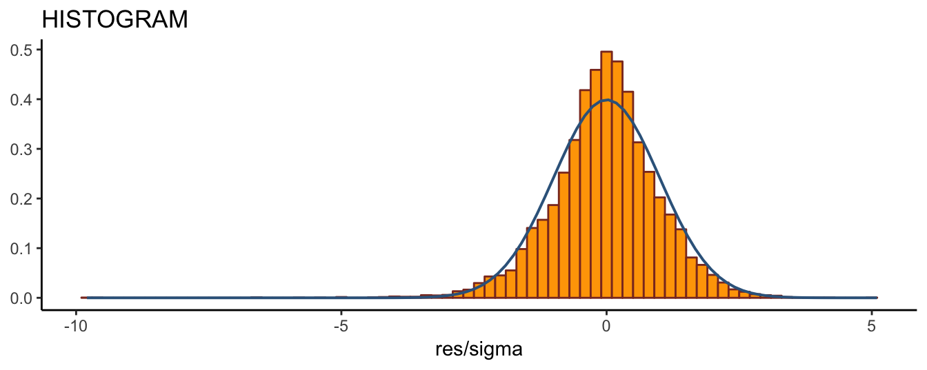
Figure 5.11: Histogram of the standardized residuals and the standard normal distribution.
We can also consider the auto-correlation of residuals and square residuals to assess if there is neglected dependence in the conditional mean and variance and the ACF are shown in Figure 5.12. Overall, there is weak evidence of auto-correlation in the standardized residuals and in their squares, so that, from this standpoint, the GARCH(1,1) model seems to be well specified to model the daily returns of the S&P 500.
p1 <- ggacf((res/sigma), lag=20)
p2 <- ggacf((res/sigma)^2, lag=20)
gridExtra::grid.arrange(p1, p2, ncol=2)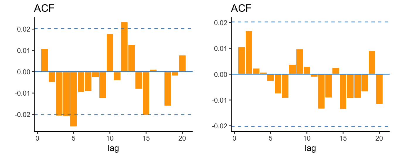
Figure 5.12: ACF of the standardized residuals of the AR(1)-GARCH(1,1) model and their square values.
Another package that provides functions to estimate a wide range of GARCH models is the rugarch package. This packages requires first to specify the functional form of the conditional mean and variance using the function ugarchspec() and then proceed with the estimation using the function ugarchfit(). Below is an example for an AR(1)-GARCH(1,1) model estimated on the daily S&P 500 returns:
library(rugarch)
spec = ugarchspec(variance.model=list(model="sGARCH",garchOrder=c(1,1)),
                  mean.model=list(armaOrder=c(1,0)))
fitgarch = ugarchfit(spec = spec, data = sp500daily)
Estimate SE
mu 0.059 7.084
ar1 0.004 0.351
omega 0.016 6.951
alpha1 0.082 13.866
beta1 0.905 129.918The estimation results are the same as those obtained for the fGarch package and more information about the estimation results can be obtained using command show(fitgarch).
The estimation of the GJR-GARCH model is quite straightforward in this package since it requires only to specify the option model='gjrGARCH' in ugarchspec(), in addition to selecting the orders for the conditional mean and variance as shown below:
spec = ugarchspec(variance.model=list(model="gjrGARCH",garchOrder=c(1,1)),
                  mean.model=list(armaOrder=c(1,0)))
fitgjr = ugarchfit(spec = spec, data = sp500daily)| Estimate | SE | |
|---|---|---|
| mu | 0.035 | 4.194 |
| ar1 | 0.009 | 0.783 |
| omega | 0.019 | 8.347 |
| alpha1 | 0.018 | 4.139 |
| beta1 | 0.904 | 131.607 |
| gamma1 | 0.121 | 11.990 |
The results for the S&P 500 confirm the earlier discussion that positive returns have a negligible effect in increasing volatility (\(\hat\alpha_1\) =0.018) while negative returns have a very large and significant effect (\(\hat\gamma_1\) = 0.121). Figure 5.13 compares the time series of the volatility estimate \(\hat{\sigma}_t\) for the GARCH and GJR models. Although the time series look pretty similar, the scatter plot shows that during turbulent times the volatility estimate of GJR is larger relative to GARCH(1,1) due to the more pronounced reaction to negative returns.
p1 <- autoplot(merge(GARCH = sigma(fitgarch), GJR = sigma(fitgjr)), scales="fixed") + theme_bw()
p2 <- ggplot(data=merge(GARCH = sigma(fitgarch), GJR = sigma(fitgjr))) +
  geom_point(aes(x = GARCH, y=GJR), color="gray70", size=0.3) +
  geom_abline(intercept=0, slope=1, color="steelblue3", linetype="dashed", size=0.8) + theme_bw()
gridExtra::grid.arrange(p1, p2, ncol=2)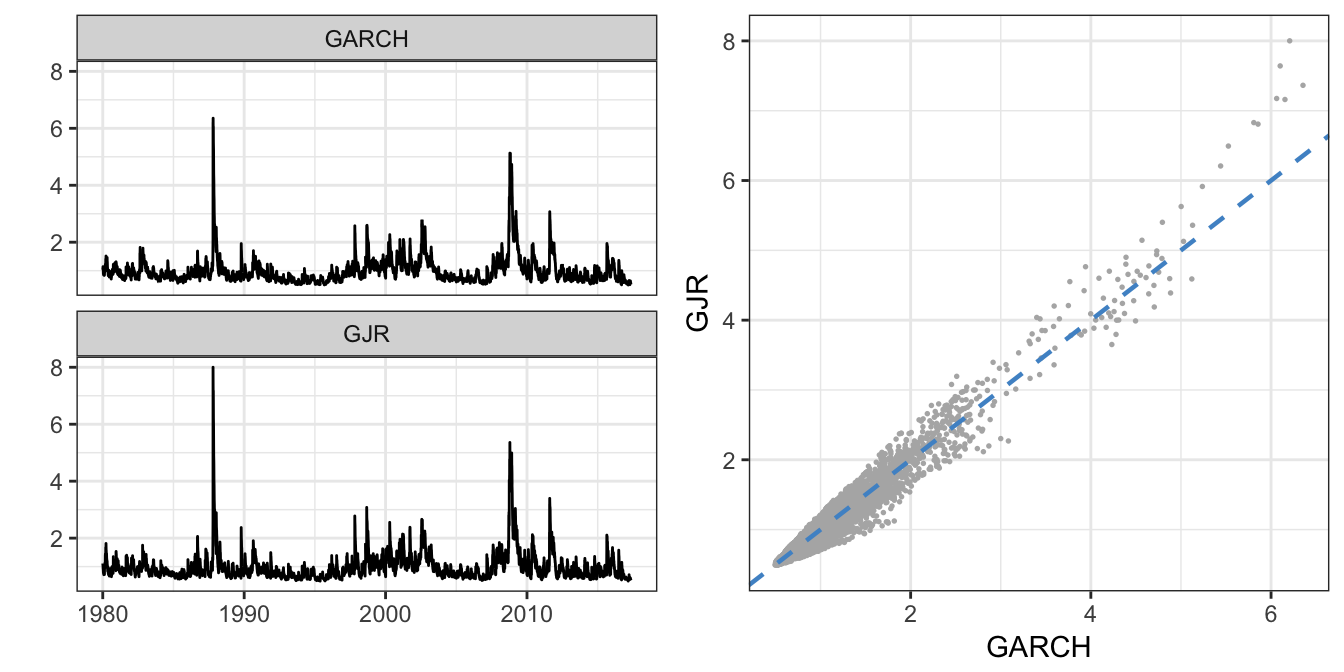
Figure 5.13: Time series of the GARCH and GJR volatility estimate (left) and their scatter plot (right).
Is this asymmetry a general feature of financial data or is it more limited to some asset classes? We can answer this question by estimating the GJR-GARCH model on the daily returns of the JPY/USD exchange rate. The estimation results for \(\gamma\) in this case provide a t-stat of 1 that is not significant even at 10% significance level thus indicating that exchange rate returns do not show the asymmetric behavior of volatility that is a features of stock returns.
| Estimate | SE | |
|---|---|---|
| mu | -0.004 | -0.582 |
| ar1 | 0.003 | 0.277 |
| omega | 0.008 | 2.605 |
| alpha1 | 0.040 | 4.182 |
| beta1 | 0.937 | 55.220 |
| gamma1 | 0.007 | 1.300 |
The selection of the best performing volatility model can be done using the AIC selection criterion, similarly to the selection of the optimal order \(p\) for AR(p) models. The package rugarch provides the function infocriteria() that calculates AIC and several other selection criteria. These criteria are different in the amount of penalization that they involve for adding more parameters (AR(1)-GJR has one parameter more than AR(1)-GARCH). For all criteria, the best model is the one that provides the smallest value. In this case the GJR specification clearly outperforms the basic GARCH(1,1) model for all criteria.
fit.ic <- cbind(infocriteria(fitgarch), infocriteria(fitgjr))
colnames(fit.ic) <- c("GARCH","GJR")
GARCH GJR
Akaike 2.67611 2.65245
Bayes 2.67991 2.65700
Shibata 2.67611 2.65245
Hannan-Quinn 2.67740 2.65399The function ugarchforecast() allows to compute the out-of-sample forecasts for a model n.ahead periods. The plot below shows the forecasts made in 2017-05-10 when the volatility estimate \(\sigma_{t+1}\) was 0.52 for GARCH and 0.517. Both models forecast an increase in volatility in the future since the volatility is mean-reverting in these models (and at the moment the forecast was made volatility was below its long-run level \(\sigma\)).
nforecast = 250
garchforecast <- ugarchforecast(fitgarch, n.ahead = nforecast)

ggplot(temp) + geom_line(aes(Date, GARCH), color="tomato3") +
  geom_line(aes(Date, GJR), color="steelblue2") +
  geom_hline(yintercept = sd(sp500daily), color="seagreen4", linetype="dashed") +
  labs(x=NULL, y=NULL, title="Volatility forecasts",
       subtitle=paste("Forecast date: ", end(sp500daily))) + theme_bw()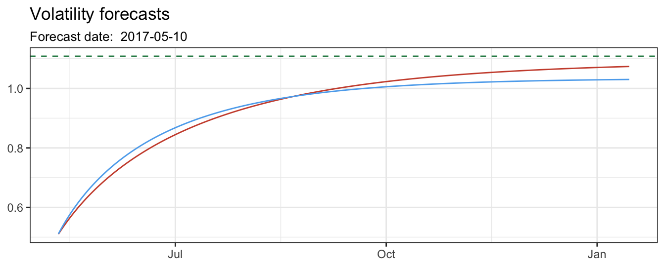
Figure 5.14: Volatility forecasts from 1 to 250 days ahead. The horizontal line represents the unconditional standard deviation of the returns.
Finally, we can compare the GARCH and GJR specifications based on the effect of a shock (\(\epsilon_{t}\)) on the conditional variance (\(\sigma^2_t\)). The left plot refers to the GARCH(1,1) model and clearly show that positive and negative shocks (of the same magnitude) increase the conditional variance by the same amount. However, the news impact curve for the GJR model clearly shows the asymmetric effect of shocks, since there is no effect when \(\epsilon_{t-1}\) is positive but a large effect when the shock is negative.
newsgjr   <- newsimpact(fitgjr)
p1 <- qplot(newsgarch$zx, newsgarch$zy, geom="line", main="GARCH") +
  geom_vline(xintercept = 0, linetype="dashed") + theme_bw()
p2 <- qplot(newsgjr$zx, newsgjr$zy, geom="line", main="GJR") +
  geom_vline(xintercept = 0, linetype="dashed") + theme_bw()
gridExtra::grid.arrange(p1, p2, ncol=2)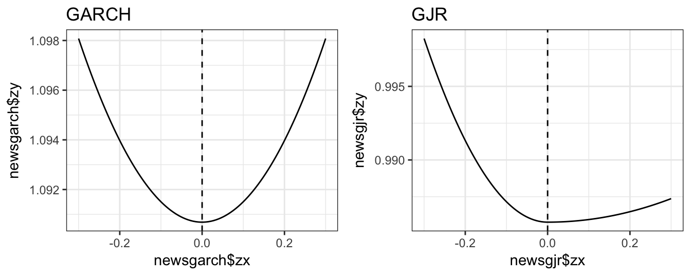
Figure 5.15: News Impact Curve (NIC) for the GARCH and GJR models.
R commands
| FUNCTIONS | PACKAGES |
|---|---|
| rollmean() | zoo |
| SMA() | TTR |
| EMA() | tseries |
| garch() | fGarch |
| garchFit() | rugarch |
| ugarchspec() | |
| ugarchfit() | |
| ugarchforecast() | |
| newsimpact() |
Exercises
- Exercise 1
- Exercise 2
References
Engle, Robert F. 1982. “Autoregressive Conditional Heteroscedasticity with Estimates of the Variance of United Kingdom Inflation.” Econometrica, 987–1007.
More generally, if \(\mu_{t+1} \not= 0\) then the conditional variance is a function of the current and past values of \(\eta_t^2\) rather than \(R^2_{t}\).↩
Furthermore, the volatility is not directly observable which does not allow the OLS estimation of the conditional variance model as it would be the case if the dependent variable is observable. However, recent advances in financial econometrics that will be discussed in the following Chapter have partly overcome this difficulty.↩