7 Measuring Financial Risk

The emergence of derivatives in the 1980s and several bankruptcies due to their misuse led the financial industry and regulators to develop rules to measure the potential portfolio losses in adverse market conditions. One of the goals of these efforts was to provide banks with a framework to determine the capital needed to survive during periods of economic and financial distress. Measuring risk is a necessary condition for managing risk: institutions need to be able to quantify the amount of risk they face to effectively elaborate a strategy to mitigate the consequences of extreme negative events. The aim of this Chapter is to discuss the application of some methods that have been proposed to measure financial risk, in particular market risk which represents the potential losses deriving from adverse movements of equity or currency markets, interest rates etc.

7.1 Value-at-Risk (VaR)

The VaR methodology was introduced in the early 1990s by the investment bank J.P. Morgan to measure the minimum portfolio loss that an institution might face if an unlikely adverse event occurred at a certain time horizon. Let’s define the profit/loss of a financial institution in day \(t+1\) by \(R_{t+1} = 100 * ln(W_{t+1}/W_t)\), where \(W_{t+1}\) is the portfolio value in day \(t+1\). Then Value-at-Risk (VaR) at \(100(1-\alpha)\)% is defined as

\[ P(R_{t+1} \leq VaR^{1-\alpha}_{t+1}) = \alpha \]

where the typical values of \(\alpha\) are 0.01 and 0.05. In practice, \(VaR^{1-\alpha}_{t+1}\) is calculated every day and for an horizon of 10 days (2 trading weeks). If \(VaR^{1-\alpha}_{t+1}\) is expressed in percentage return it can be easily transformed into dollars by multiplying the portfolio value in day \(t\) (denoted by \(W_{t}\)) with the expected loss, that is, \(VaR^{1-\alpha}_{t+1} = W_{t} * (exp(VaR^{1-\alpha}_{t+1}/100)-1)\). From a statistical point view, 99% VaR represents the 1% quantile, that is, the value of \(R_{t+1}\) such that there is only 1% probability that the random variable takes a value smaller or equal to that value. The graphs below shows the Probability Density Function (PDF) and the Cumulative Distribution Function (CDF). Risk calculation is devoted to the left tail of the return distribution since it represents large and negative outcomes for the portfolio of financial institutions. This is the reason why the profession has devoted a lot of energy to make sure that the left tail, rather than the complete distribution, is appropriately specified since a poor model for the left tail implies poor risk estimates (poor in a sense that will become clear in the backtesting section).

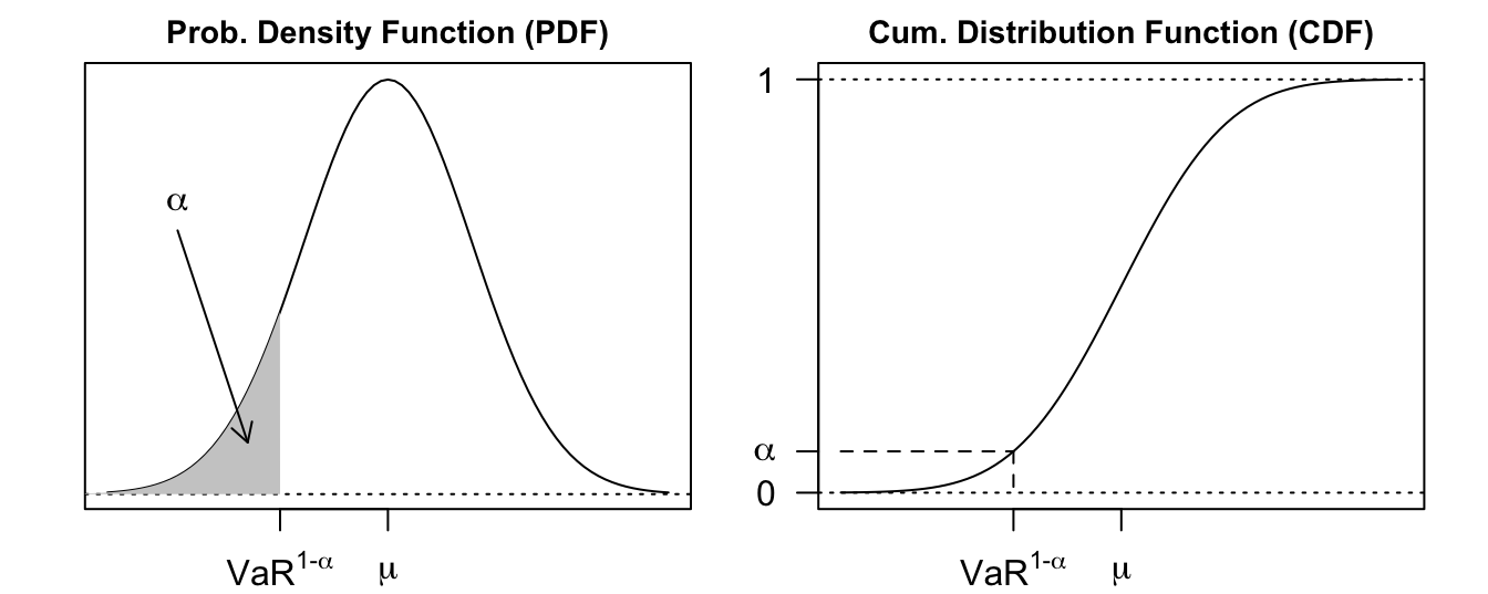
Figure 7.1: The Probability Density Function (PDF) and Cumulative Distribution Function (CDF) for a normal distribution with mean \(\mu\) and variance \(\sigma^2\). Value at Risk (\(VaR^{1-\alpha}\)) at \(1-\alpha\) level represents the \(\alpha\) quantile of the distribution.

7.1.1 VaR assuming normality

Calculating VaR requires making an assumption about the distribution of the profit/loss of the institution. The simplest and most familiar assumption we can introduce is that \(R_{t+1} \sim N(\mu, \sigma^2)\), where \(\mu\) represents the mean of the distribution and \(\sigma^2\) its variance. The assumption is equivalent to assume that the profit/loss follows the model \(R_{t+1} = \mu + \sigma\epsilon_{t+1}\), with \(\epsilon_{t+1} \sim N(0,1)\). The quantiles for this model are given by \(\mu + z_{\alpha}\sigma\), where \(\alpha\) is the probability level and \(z_{\alpha}\) represents the \(\alpha\) quantile of the standard normal distribution. The typical levels of \(\alpha\) for VaR calculations are 1 and 5% and the corresponding \(z_{\alpha}\) are -1.64 and -2.33, respectively. Hence, 99% VaR under normality is obtained as follows: \[ VaR^{0.99}_{t+1} = \mu - 2.33 * \sigma \] As an example, assume that an institution is holding a portfolio that replicates the S&P 500 Index and wants to calculate the 99% VaR for this position. If we assume that returns are normally distributed, then to calculate \(VaR^{0.99}_{t+1}\) we need to estimate the expected daily return of the portfolio (i.e., \(\mu\)) and its expected volatility (i.e., \(\sigma\)). Let’s assume that we believe that the distribution is approximately constant over time so that we can estimate the mean and standard deviation of the returns over a long period of time. In the illustration below we use the S&P 500 time series that was used in the volatility chapter that consists of daily returns from 1990 to 2017 (6893 observations).

mu    = mean(sp500daily)
sigma = sd(sp500daily)
var   = mu + qnorm(0.01) * sigma

[1] -2.569

The 99% VaR is -2.569% and represents the minimum loss of holding the S&P500 for the following day with 1% (or smaller) probability. If we use a shorter estimation window of one year (252 observations), the \(VaR\) estimation would be -1.778%. The difference between the two VaR estimates is quite remarkable given that we only changed the size of the estimation window. The standard deviation declines from 1.119% in the full sample to 0.786% in the shorter sample, whilst the mean changes from 0.034% to 0.051%. As discussed in the volatility modeling Chapter, it is extremely important to account for time variation in the distribution of financial returns if the interest is to estimate VaR at short horizons (e.g., a few days ahead).

7.1.2 Time-varying VaR

So far we assumed that the mean and standard deviation of the return distribution are constant and represent the long-run distribution of the variable. However, this might not be the best way to predict the distribution of the profit/loss at very short horizons (e.g., 1 to 10 days ahead) if the return volatility changes over time. In particular, in the volatility chapter we discussed the evidence that the volatility of financial returns changes over time and introduced models to account for this behavior. We can model the conditional distribution of the returns in day \(t+1\) by assuming that both \(\mu_{t+1}\) and \(\sigma_{t+1}\) are time-varying conditional on the information available in day \(t\). Another decision that we need to make is the distribution of the errors. We can assume, as above, that the errors are normally distributed so that 99% VaR is calculated as: \[ VaR^{0.99}_{t+1} = \mu_{t+1} - 2.33 * \sigma_{t+1} \] where the expected return \(\mu_{t+1}\) can be either constant (i.e. \(\mu_{t+1} = \mu\)), or an AR(1) process (\(\mu_{t+1} = \phi_0 + \phi_1 * R_{t}\)), and the conditional variance can be modeled as MA, EMA, or with a GARCH-type model. In the example below, I assume that the conditional mean is constant (and equal to the sample mean) and model the conditional variance of the demeaned returns as an EMA with parameter \(\lambda = 0.06\):

library(TTR)
mu       <- mean(sp500daily) 
sigmaEMA <- EMA((sp500daily-mu)^2, ratio=0.06)^0.5
var      <- mu + qnorm(0.01) * sigmaEMA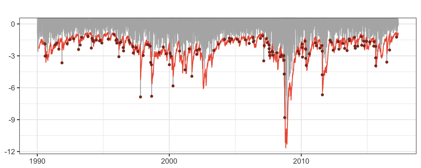

Figure 7.2: 99% VaR for the daily returns of the SP 500 Index. The dots represent the days in which the returns were smaller than VaR, also called violations or hits.

The VaR time series shows in Figure 7.2 inherits the characteristic of the volatility of alternating between calm periods of low volatility and risk, and other periods of increased uncertainty and potentially large losses. For this example, we find that in 2.089% of the 6893 days the return was smaller relative to VaR. Since we calculated VaR at 99% we expected to experience only 1% of days with violations and the difference between the sample and population value might indicate that the risk model might be misspecified. We will discuss the properties of the violations for a risk model in the section devoted to backtesting.

7.1.3 Expected Shortfall (ES)

VaR represents the maximum (minimum) loss that is expected with, e.g., 99% (1%) probability. However, it can be criticized on the ground that it does not convey the information of the potential loss that is expected if indeed an extreme event (only likely 1% of less) occurs. For example, a VaR of -5.52% provides no information on how large the portfolio loss is expected to be if the portfolio return will happen to be smaller than VaR. That is, how large do we expect the loss be in case VaR is violated? A risk measure that quantifies this potential loss is Expected Shortfall (ES) which is defined as \[ES^{1-\alpha}_{t+1} = E(R_{t+1}|R_{t+1} \leq VaR^{1-\alpha}_{t+1})\] that is, the expected portfolio return conditional on being on a day in which the return is smaller than VaR. This risk measure focuses its attention on the left tail of the distribution and it is highly dependent on the shape of the distribution in that area, while it neglects all other parts of the distribution.

An analytical formula for ES is available if we assume that returns are normally distributed. In particular, if \(R_{t+1}=\sigma_{t+1}\epsilon_{t+1}\) with \(\epsilon_{t+1} \sim N(0,1)\), then VaR is calculated as \(VaR^{1-\alpha}_{t+1} = z_{\alpha}\sigma_{t+1}\). The conditioning event is that the return in the following day is smaller than VaR and the probability of this event happening is \(\alpha\), e.g. 0.01. We then need to calculate the expected value of \(R_{t+1}\) over the interval from minus infinity to \(R_{t+1}\) which corresponds to a truncated normal distribution with density function given by \(f(R_{t+1}|R_{t+1} \leq VaR^{1-\alpha}_{t+1}) = \phi(R_{t+1}) /\Phi(VaR^{1-\alpha}_{t+1}/\sigma_{t+1})\), where \(\phi(\cdot)\) and \(\Phi(\cdot)\) represent the PDF and the CDF of the normal distribution (i.e., \(\Phi(VaR^{1-\alpha}_{t+1}/\sigma_{t+1})=\Phi(z_{\alpha}) =\alpha\)). We can thus express ES as \[ ES^{1-\alpha}_{t+1} = - \sigma_{t+1} \frac{\phi(z_{\alpha})}{\alpha} \] where \(z_{\alpha}\) is equal to -2.33 and -1.64 for \(\alpha\) equal to 0.01 and 0.05, respectively. If we are calculating VaR at 99% so that \(\alpha\) is equal to 0.01 then ES is equal to \[ ES^{0.99}_{t+1} = - \sigma_{t+1} \frac{\phi(-2.33)}{0.01} = -2.64 \sigma_{t+1} \] where the value \(-2.64\) can be obtained in R typing the command (2*pi)^(-0.5) * exp(-(2.33^2)/2) / 0.01 or using the function dnorm(-2.33) / 0.01. If \(\alpha = 0.05\) then the constant to calculate ES is -2.08 instead of -1.64 for VaR. Hence, ES leads to more conservative risk estimates since the expected loss in a day in which VaR is exceeded is always larger than VaR. This is shown in Figure 7.3 where the difference between VaR and ES is plotted as a function of \(1-\alpha\):

sigma = 1
alpha = seq(0.001, 0.05, by=0.001)
ES    =  - dnorm(qnorm(alpha)) / alpha * sigma
VaR   = qnorm(alpha) * sigma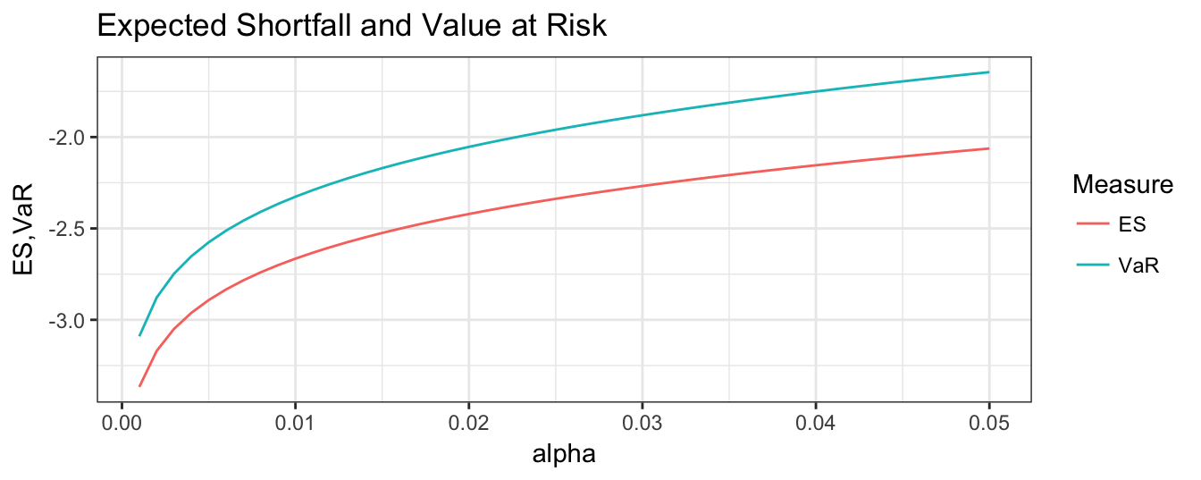

Figure 7.3: Comparison of the ES and VaR risk measures under the assumption of normally distributed profit/loss at different values of \(\alpha\).

7.1.4 \(\sqrt{K}\) rule

The Basel Accords require VaR to be calculated at a horizon of 10 days and for a risk level of 99%. In addition, the Accords allow financial institution to scale up the 1-day VaR to the 10 day horizon by multiplying it by \(\sqrt{10}\). Why \(\sqrt{10}\)? Under what conditions is the VaR for the cumulative returns over 10 days, denoted by \(VaR_{t+1:t+10}\), equal to \(\sqrt{10} * VaR_{t+1}\)?

In day \(t\) we are interested in calculating the risk of holding the portfolio over a horizon of \(K\) days, that is, assuming that we can liquidate the portfolio only on the \(K\)th day. Regulators require banks to use \(K=10\) that corresponds to two trading weeks. To calculate risk of holding the portfolio in the next \(K\) days we need to obtain the distribution of the sum of \(K\) daily returns or cumulative return, denoted by \(R_{t+1:t+k}\), which is given by \(\sum_{k=1}^K R_{t+k} = R_{t+1} + \cdots + R_{t+K}\), where \(R_{t+k}\) is the return in day \(t+k\). If we assume that these daily returns are independent and identically distributed (i.i.d.) with mean \(\mu\) and variance \(\sigma^2\), then the expected value of the cumulative return is \[ E\left( \sum_{k=1}^K R_{t+k}\right) = \sum_{k=1}^K \mu = K\mu \] and its variance is \[ Var\left( \sum_{k=1}^K R_{t+k} \right) = \sum_{k=1}^K \sigma^2 = K \sigma^2 \] so that the standard deviation of the cumulative return is equal to \(\sqrt{K}\sigma\). If we maintain the normality assumption that we introduced earlier, than the 99% \(VaR\) of \(R_{t+1:t+K}\) is given by \[ VaR^{1-\alpha}_{t+1:t+K} = K\mu -2.33 \sqrt{K}\sigma \] In this formula, the mean and standard deviation are estimated on daily returns and they are then scaled up to horizon \(K\).

This result relies on the assumption that returns are serially independent which allows us to set all covariances between returns in different days equal to zero in the formula for the variance. The empirical evidence from the ACF of daily returns indicates that this assumption is likely to be accurate most of the time, although in times of market booms or busts returns could be, temporarily, positively correlated. What would be the effect of positive correlation in returns on VaR? The first-order covariance can be expressed in terms of correlation as \(\rho\sigma^2\), with \(\rho\) representing the first order serial correlation. To keep things simple, assume that we are interested in calculating VaR for the two-day return, that is, \(K=2\). The variance of the cumulative return is \(Var(R_{t+1} + R_{t+2})\) which is equal to \(Var(R_{t+1}) + Var(R_{t+2}) + 2 Cov(R_{t+1},R_{t+2}) = \sigma^2 + \sigma^2 + 2\rho\sigma^2\). This can be re-written as \(2\sigma^2(1+\rho)\) which shows that in the presence of positive correlation \(\rho\) the cumulative return becomes riskier, relative to the independent case, since \(2\sigma^2(1+\rho) > 2\sigma^2\). The Value-at-Risk for the two-day return is then \(VaR^{0.99}_{t+1:t+2} = 2\mu -2.33 * \sigma * \sqrt{2}\sqrt{1+\rho}\), which is smaller relative to the VaR assuming independence that is given by \(2\mu -2.33 *\sigma * \sqrt{2}\). Hence, neglecting positive correlation in returns leads to underestimating risk and the potential portfolio loss deriving from an extreme (negative) market movement.

7.1.5 VaR assuming non-normality

One of the stylized facts of financial returns is that the empirical frequency of large positive/negative returns is higher relative to the frequency we would expect if returns were normally distributed. This finding of fat tails in the return distribution can be partly explained by time-varying volatility: the extreme returns are the outcome of a regime of high volatility that occurs occasionally, although most of the time returns are in a calm period with low volatility. The effect of mixing periods of high and low volatility is that the (unconditional) volatility estimate based on the full sample overestimates uncertainty when volatility is low, and underestimates it in turbulent times. This can be illustrated with a simple example: assume that in 15% of days volatility is high and equal to 5% while in the remaining 85% of the days it is low and equal to 0.5%. Average volatility based on all observations is then 0.15 * 5 + 0.85 * 0.5 = 1.175%. This implies that in days of high volatility, the returns appear large relative to a standard deviation of 1.175% although they are normal considering that they belong to the high volatility regimes with a standard deviation of 5. On the other hand, the bulk of returns belong to the low volatility regime which looks like a concentration of small returns relative to the average volatility of 1.175%.

To evaluate the evidence of deviation from normality, we can calculate the sample skewness and excess kurtosis for the standardized residuals and compare them to the their theoretical value of 0. The skewness of the returns standardized by the EMA volatility estimate is -0.167 and the excess kurtosis is estimated equal to 0.101. Both statistics indicate that the standardized residuals are not close to normality due to the presence of large residuals (kurtosis) in the left tail of the distribution (skewness). This evidence is very important for risk measurement which is mostly concerned with the far left of the distribution: time-variation in volatility is the biggest factor driving non-normality in returns so that when we calculate risk measures we are confident that a combination of the normal distribution and a dynamic method to forecast volatility should provide reasonably accurate VaR estimates. However, we still might want to account for the non-normality in the standardized returns \(\epsilon_t\) and we will consider two possible approaches in this Section.

One approach to relax the assumption of normally distributed errors is the Cornish-Fisher approximation which consists of performing a Taylor expansion of the normal distribution around its mean. This has the effect of producing a distribution which is a function of skewness and kurtosis. We skip the mathematical details of the derivation and focus on the VaR calculation when this approximation is adopted. If we assume the mean \(\mu\) is equal to zero, the 99% VaR for normally distributed returns is calculated as \(-2.33 * \sigma_{t+1}\) or, more generally, by \(z_{\alpha} \sigma_{t+1}\) for \(100(1-\alpha)\)% VaR, where \(z_{\alpha}\) represents the \(1-\alpha\)-quantile of the standard normal distribution. With the Cornish-Fisher (CF) approximation VaR is calculated in a similar manner, that is, \(VaR^{1-\alpha}_{t+1} = z^{CF}_{\alpha}\sigma_{t+1}\), with the quantile \(z^{CF}_{\alpha}\) calculated as follows: \[ z^{CF}_{\alpha} = z_{\alpha} + \frac{SK}{6}\left[z_{\alpha}^2 - 1\right] + \frac{EK}{24} \left[z_{\alpha}^3 - 3z_{\alpha}\right] + \frac{SK^2}{36} \left[ 2z_{\alpha}^5 - 5 z_{\alpha} \right] \]

where \(SK\) and \(EK\) represent the skewness and excess kurtosis, respectively. If the data are normally distributed then \(SK=EK=0\) so that \(z^{CF}_{\alpha} = z_{\alpha}\). However, in case the distribution is asymmetric and/or with fat tails the effect is that \(z^{CF}_{\alpha} \leq z_{\alpha}\). In practice, we estimate the skewness and the excess kurtosis from the sample and use those values to calculate the quantile for VaR calculations. Figure 7.4 we show the quantile \(z^{CF}_{0.01}\) and its relationship to \(z_{0.01}\) as a function of the skewness and excess kurtosis parameters. The left plot shows the effect of the skewness parameter on the quantile, while holding the excess kurtosis equal to zero. Instead, the plot on the right shows the effect of increasing values of excess kurtosis, while the skewness parameter is kept constant and equal to zero. As expected, the \(z^{CF}_{0.01}\) is smaller than \(z_{0.01} = -2.33\) and it is interesting to notice that negative skewness increases the (absolute) value of \(z^{CF}_{0.01}\) more than positive skewness of the same magnitude. This is due to the fact that negative skewness implies a higher probability of large negative returns compared to large positive returns. The effect on VAR of accounting for asymmetry and fat tails in the data is thus to provide more conservative risk measures.

alpha = 0.01
# case 1: skewness holding excess kurtosis equal to 0
EK = 0; SK = seq(-1, 1, by=0.05)
z = qnorm(alpha)
zCF = z + (SK/6) * (z^2 - 1) + (EK/24) * (z^3 - 3 * z) + 
  (SK^2/36) * (2*z^5 - 5*z)
q1 <- ggplot() + geom_line(aes(SK,zCF), color="seagreen4") + 
      labs(x="Skewness", y=expression(z[alpha])) + 
      geom_hline(yintercept=rep(z, length(SK)), linetype="dashed", size=1.2) + theme_bw() +
      coord_cartesian(y=c(-7.1, -1.9))
# case 2: kurtosis holding skewness equal to 0
EK1 = seq(0, 10,by=0.1); SK1 = 0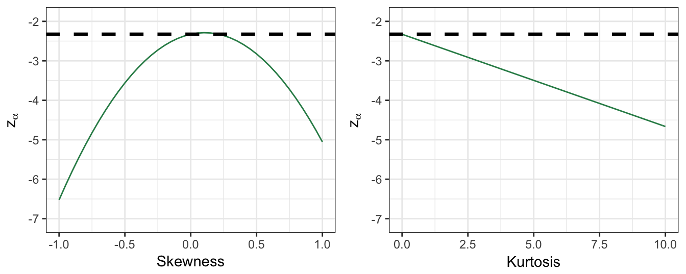

Figure 7.4: The effect of skewness and kurtosis on the critical value used in the Cornish-Fisher approximation approach.

An alternative approach to allow for non-normality is to make a different distributional assumption for \(\epsilon_{t+1}\) that captures the fat-tailness in the data. A distribution that is often considered is the \(t\) distribution with a small number of degrees of freedom. Since the \(t\) distribution assigns more probability to events in the tail of the distribution, it will provide more conservative risk estimates relative to the normal distribution. Figure 7.5 shows the \(t\) distribution for 4, 10, and \(\infty\) degree-of-freedom, while the plot on the right zooms on the shape of the left tail of these distributions. It is clear that the smaller the d.o.f used the more likely are extreme events relative to the standard normal distribution (\(d.o.f.=\infty\)). So, also this approach delivers more conservative risk measures relative to the normal distribution since it assigns higher probability to extreme events.

q1 <- ggplot(data.frame(x = c(-8, 8)), aes(x = x)) +
        stat_function(fun = dnorm, aes(colour = "N(0,1)")) +
        stat_function(fun = dt, args = list(df=4),  aes(colour = "t(4)")) +
        stat_function(fun = dt, args = list(df=10),  aes(colour = "t(10)")) + 
        theme_bw() + labs(x = NULL, y= NULL) + coord_cartesian(x=c(-3,3)) +
        scale_colour_manual("Distribution", values = c("seagreen3", "steelblue3", "tomato3")) + 
        theme(legend.position="bottom")
q2 <- q1 + coord_cartesian(x=c(-8, -3), y=c(0,0.03))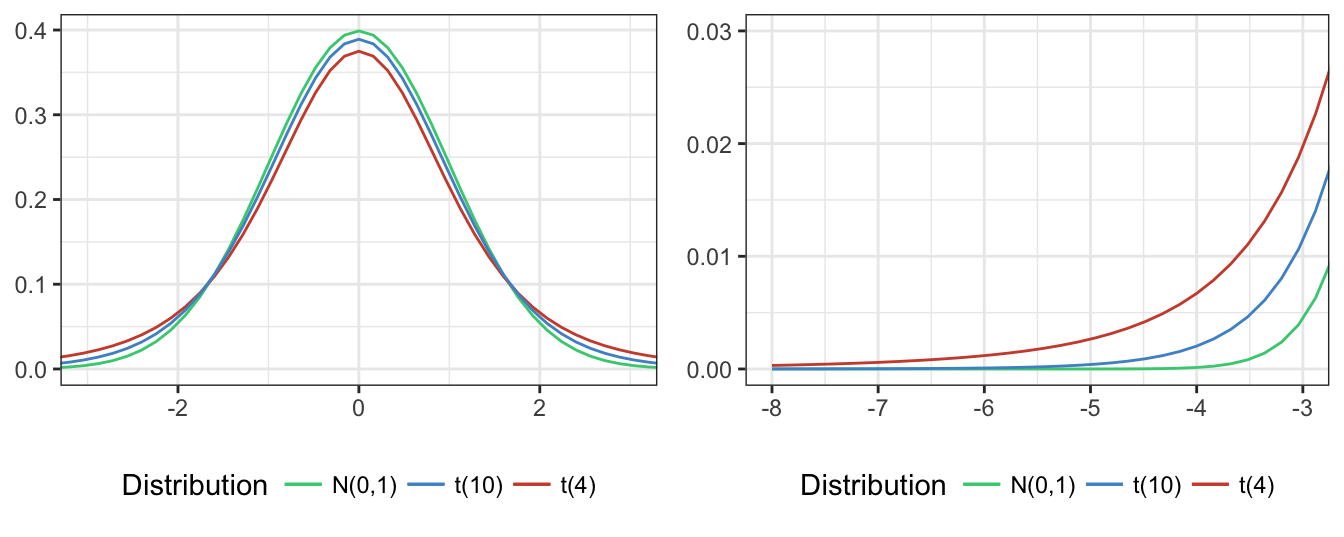

Figure 7.5: Comparison of the standard normal distribution and t distribution with 4 and 10 degree-of-freedom. The right plot zooms on the left tail of the three distributions.

To be able to use the \(t\) distribution for risk calculation we need to estimate the degree-of-freedom parameter, denoted by \(d\). In the context of a GARCH volatility model this can be easily done by considering \(d\) as an additional parameter to be estimated by maximizing the likelihood function based on the assumption that the \(\epsilon_{t+1}\) shocks follow a \(t_d\) distribution. A simple alternative approach to estimate the degree-of-freedom parameter \(d\) exploits the fact that the excess kurtosis of a \(t_d\) distribution is equal to \(EK = 6/(d-4)\) (for \(d>4\)) which is only a function of the parameter \(d\). Thus, based on the sample excess kurtosis we can then back out an estimate of \(d\). The steps are as follows:

1. estimate by ML the GARCH model assuming that the errors are normally distributed (or using EMA)
2. calculate the standardized residuals as \(\epsilon_{t+1} = R_{t+1} / \sigma_{t+1}\)
3. estimate the excess kurtosis of the standardized residuals and obtain \(d\) as \(d = 6/EK + 4\)

For the standardized returns of the S&P 500 the sample excess kurtosis is equal to 2.262 so that the estimate of \(d\) is equal to approximately 7 which indicates the need for a fat-tailed distribution. In practice, it would be advisable to estimate the parameter \(d\) jointly with the remaining parameters of the volatility model, rather than separately. Still, this simple approach provides a starting point to evaluate the usefulness of fat tailed distributions in risk measurement.

7.2 Historical Simulation (HS)

So far we discussed methods to calculate VaR that rely on choosing a probability distribution and a volatility model. A distributional assumption we made is that returns are normal, which we later relaxed by introducing the Cornish-Fisher approximation and the \(t\) distribution. In terms of the volatility model, we considered several possible specifications such as EMA, GARCH, and GJR-GARCH, which we can compare using selection criteria.

An alternative approach that avoids making any assumption and let the data speak for itself is represented by Historical Simulation (HS). HS consists of calculating the empirical quantile of returns at \(100*\alpha\)% level based on the most recent M days. This approach is called non-parametric because it estimates 99% VaR to be the value such that 1% of the more recent M returns are smaller than, without introducing assumptions on the return distribution and the volatility structure. In addition to its flexibility, HS is very easy to compute since it does not require the estimation of any parameter for the volatility model and the distribution. However, there are also a few difficulties in using HS to calculate risk measures. One issue is the choice of the estimation window size M. Practitioners often use values between M=250 and 1000, but, similarly to the choice of smoothing in MA and EMA, this is an ad hoc value that has been validated by experience rather than being optimally selected based on a criterion. Another complication is that HS applied to daily returns provides a VaR measure at the one day horizon which, for regulatory purposes, should then be converted to a 10-day horizon. What is typically done is to apply the \(\sqrt{10}\) rule discussed before, although it does not have much theoretical justification in the context of HS since we are not actually making any assumption about the return distribution. An alternative would be to calculate VaR as the 1% quantile of the (non-overlapping) cumulative return instead of the daily return. However, this would imply a much smaller sample size, in particular for small M.

The implementation in R is quite straightforward and shown below. The function quantile() calculates the \(1-\alpha\) quantile for a return series which we can combine with the function rollapply() from package zoo to apply it recursively to a rolling window of size M. For example, the command rollapply(sp500daily, 250, quantile, probs=alpha, align="right") calculates the function quantile (for probs=alpha and alpha=0.01) for the sp500daily time series with the first VaR forecast for day 251 until the end of the sample. Figure 7.6 compares VaR calculated with the HS method for an estimation window of 250 and 1000 days. The shorter estimation window makes the VaR more sensitive to market events as opposed to M=1000 that changes very slowly. A characteristic of HS for M=1000 is that it is constant for long periods of time, even though volatility might have significantly decreased for several months.

M1 = 250
M2 = 1000
alpha = 0.01
hs1 <- rollapply(sp500daily, M1, quantile, probs=alpha, align="right")
hs2 <- rollapply(sp500daily, M2, quantile, probs=alpha, align="right")

mydata <- merge(hs1, hs2) %>% fortify %>%
  tidyr::gather(Variable, Value, -Index)

ggplot() + geom_line(aes(index(sp500daily), sp500daily), color="gray70") + 
  geom_line(data=mydata, aes(Index, Value, color=Variable), size=1.2) + 
  coord_cartesian(y=c(min(sp500daily, na.rm=T), 0)) + theme_bw() + 
  labs(x=NULL, y=NULL, title="Historical Simulation") + theme(legend.position="bottom")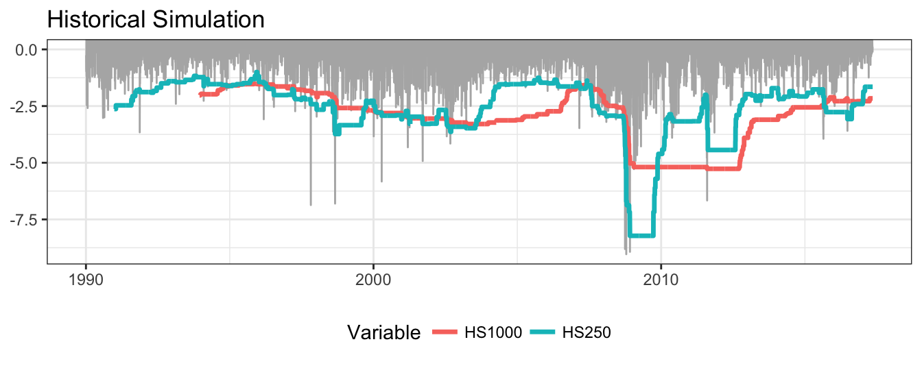

Figure 7.6: Returns and 99% VaR for the Historical Simulation (HS) method with parameter M set to 250 and 1000 days.

How good is the risk model? One metric that is used as an indicator of goodness of the risk model is the frequency of returns that are smaller than VaR, that is, \(\sum_{t=1}^T I(R_{t+1} \leq VaR_{t+1}) / T\), where \(T\) represents the total number of days and \(I(\cdot)\) denotes the indicator function. A good risk model should have the frequency of violations or hits close to the level \(1-\alpha\) for which VaR is calculated. If we are calculating VaR at 99% then we would expect that the model shows (approximately) 1% violations. For HS above, we have that for VaR calculated on the 250 window there are 1.32% of days that represent violations. For the longer window of M=1000 the violations of VaR represents 1.291% of the sample. For HS, we thus find that they are larger than expected and in the backtesting Section we will evaluate if the difference from the theoretical value of 1% is statistically significant.

In Figure 7.7, the VaR calculated from HS is compared to the EMA forecast. Although the VaR level and the dynamics is quite similar, HS changes less rapidly and remains constant for long periods of time, in particular in periods of rapid changes in market volatility.

library(TTR)
ema <- - 2.33 * EMA(sp500daily^2, ratio=0.06)^0.5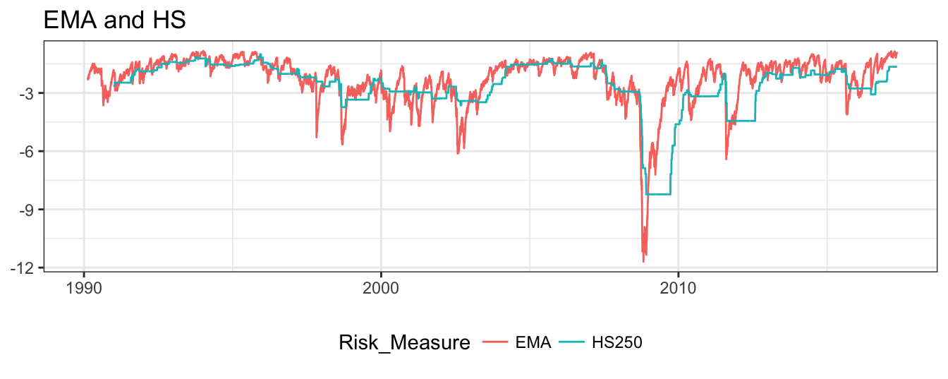

Figure 7.7: 99% VaR for the SP 500 based on the HS(250) and EMA(0.06) methods.

7.3 Simulation Methods

We discussed several approaches that can be used to calculate VaR based on parametric assumptions or that are purely non-parametric in nature. In most cases we demonstrated the technique by forecasting Value-at-Risk at the 1-day horizon. However, for regulatory purposes the risk measure should be calculated at a horizon of 10 days. An approach that is widely used by practitioners and that is also allowed by regulators is to scale up the 1-day VaR to 10-day by multiplying it by \(\sqrt{10}\).

An alternative is to use simulation methods that generate artificial future returns based on the risk model. The model makes assumptions about the volatility model, and the distribution of the error term. Using simulations we are able to produce a large number of future possible paths for the returns that are conditional on the current day. In addition, it becomes very easy to obtain the distribution of cumulative returns by summing daily simulated returns along a path. We will consider two popular approaches that differ in the way simulated shocks are generated: Monte Carlo Simulation (MC) consists of iterating the volatility model based on shocks that are simulated from a certain distribution (normal, \(t\) or something else), and Filtered Historical Simulation (FHS) that assumes the shocks are equal to the standardized returns and takes random sample of those values. The difference is that FHS does not make a parametric assumption for the \(\epsilon_{t+1}\) (similarly to HS), while MC does rely on such assumption.

7.3.1 Monte Carlo Simulation

At the closing of January 22, 2007 and September 29, 2008 the risk manager needs to forecast the distribution of returns from 1 up to K days ahead, including the cumulative or multi-period returns over these horizons. The model for returns is \(R_{t+1} = \sigma_{t+1}\epsilon_{t+1}\), where \(\sigma_{t+1}\) is the volatility forecast based on the information available up to that day. The \(\epsilon_{t+1}\) are the random shocks that the risk manager assumes are normally distributed with mean 0 and variance 1. A Monte Carlo simulation of the future distribution of the portfolio returns requires the following steps:

1. Estimation of the volatility model: we assume that \(\sigma_{t+1}\) follows a GARCH(1,1) model and estimate the model by ML using all observations available up to and including that day. Below is the code to estimate the model using the rugarch package. The volatility forecast for the following day is 0.483% which is significantly lower relative to the sample standard deviation from January 1990 to January 2007 of 0.993%. To use some terminology introduced earlier, the conditional forecast (0.483%) is lower relative to the unconditional forecast (0.993%).

  lowvol   = as.Date("2007-01-22") 
  spec     = ugarchspec(variance.model=list(model="sGARCH",garchOrder=c(1,1)),
                  mean.model=list(armaOrder=c(0,0), include.mean=FALSE))
  fitgarch = ugarchfit(spec = spec, data = window(sp500daily, end=lowvol)) 
  gcoef <- coef(fitgarch)
  sigma <- ugarchforecast(fitgarch, n.ahead=1)@forecast$sigmaFor

 omega alpha1  beta1 
 0.005  0.054  0.942 
    2007-01-22
T+1      0.483

2. The next step consists of simulating a large number of return paths, say \(S\), that are consistent with the model assumption that \(R_{t+1} = \sigma_{t+1}\epsilon_{t+1}\). This is done by generating values for the error term \(\epsilon_{t+1}\) from a certain distribution and multiply these values by the forecast \(\sigma_{t+1} =\) 0.483. Generating random variables can be easily done in R using the command rnorm() which returns random values from the standard normal distribution (and rt() does the same for the \(t\) distribution). Denote by \(\epsilon_{s,t+1}\) the \(s\)-th simulated value of the shock (for \(s=1,\cdots, S\)), then the \(s\)-th simulated value of the return is produced by multiplying \(\sigma_{t+1}\) and \(\epsilon_{s,t+1}\), that is, \(R_{s,t+1} = \sigma_{t+1}\epsilon_{s,t+1}\).

3. The next step is to use the simulate returns \(R_{s,t+1}\) to predict volatility next period, denoted by \(\sigma_{s,t+2}\). Since we have assumed a GARCH specification the volatility forecast is obtained by \((\sigma_{s,t+2})^2 = \omega + \alpha R_{s,t+1}^2 + \beta \sigma_{t+1}^2\) and the (simulated) returns at time \(t+2\) are obtained as \(R_{s,t+2} = \sigma_{s,t+2}\epsilon_{s,t+2}\), where \(\epsilon_{s,t+2}\) represent a new set of simulated values for the shocks in day \(t+2\).

4. Continue the iteration to calculate \(\sigma_{s,t+k}\) and \(R_{s,t+k}\) for \(k=1, \cdots, K\). The cumulative or multi-period return between \(t+1\) and \(t+k\) is then obtained as \(R_{s,t+1:t+K} = \sum_{j=1}^{k} R_{s,t+j}\).

The code below shows how a MC simulation can be performed and Figure 7.8 shows the quantiles of \(R_{s,t+k}\) as a function of \(k\) on the left plot and the quantiles of \(\sigma_{s,t+k}\) on the right plot (from 0.10 to 0.90 at intervals of 0.10 in addition to 0.05 and 0.95). The volatility is branching out from \(\sigma_{t+1}=\) 0.483 and its uncertainty increases with the forecast horizon. The green dashed line represents the average (over the simulations) volatility at horizon \(k\) that, as expected for GARCH models, tends toward the unconditional mean of volatility. Since January 22, 2007 was a period of low volatility, the graph shows that we should expect volatility to increase at longer horizons. This is also clear from the left plot where the return distribution becomes wider as the forecast horizon progresses.

set.seed(9874)

S = 10000  # number of MC simulations
K = 250   # forecast horizon

# create the matrices to store the simulated return and volatility
R     = xts(matrix(sigma*rnorm(S), K, S, byrow=TRUE), order.by=futdates)
Sigma = xts(matrix(sigma, K, S), order.by=futdates)

# iteration to calculate R and Sigma based on the previous day
for (i in 2:K)
{
  Sigma[i,]  = (gcoef['omega'] + gcoef['alpha1'] * R[i-1,]^2 + 
                  gcoef['beta1'] * Sigma[i-1,]^2)^0.5   
  R[i,]  = rnorm(S) * Sigma[i,]
}

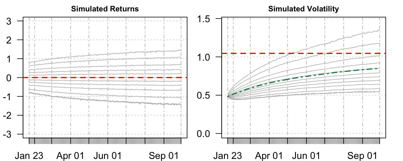
Figure 7.8: Quantiles of the simulated return and volatility distributions forecast in January 22, 2007

How would the forecasts of the return and volatility distribution look like if they were made in a period of high volatility? To illustrate this scenario we consider September 29, 2008 as the forecast base. The GARCH(1,1) forecast of volatility for the following day is 3.085% and the distribution of simulated returns and volatilities are shown in Figure 7.9. Since the day was in a period of high volatility, the assumption of stationarity of volatility made by the GARCH model implies that volatility will reduce in the future. This is clear from the return quantiles converging in the left plot, as well as from the declining average volatility in the right plot.

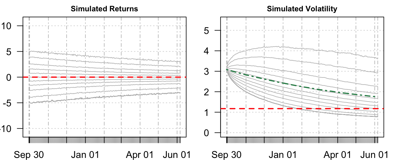
Figure 7.9: Quantiles of the simulated return and volatility distributions forecast in September 29, 2008

The cumulative or multi-period return can be easily obtained by the R command cumsum(Ret) where Ret represents the K by S matrix of simulated one-day returns that the function cumulatively sums over the columns. The outcome is also a K by S matrix with each column representing a possible path of the cumulative return from 1 to K steps ahead. Figure 7.10 shows the quantiles at each horizon \(k\) calculated across the \(S\) simulated cumulative returns. The quantile at probability 0.01 represents the 99% VaR that financial institutions are required to report for regulatory purposes (at the 10 day horizon). The left plot represents the distribution of expected cumulative returns conditional on being on January 22, 2007 while the right plot is conditional on September 29, 2008. The same scale of the \(y\)-axis for both plots highlights the striking difference in the dispersion of the distribution of future cumulative returns. Although we saw above that the volatility of daily returns is expected to increase after January 22, 2007 and decrease following September 29, 2008, the levels of volatility in these two days are so different that when accumulated over a long period of time they lead to very different distributions for the cumulative returns.

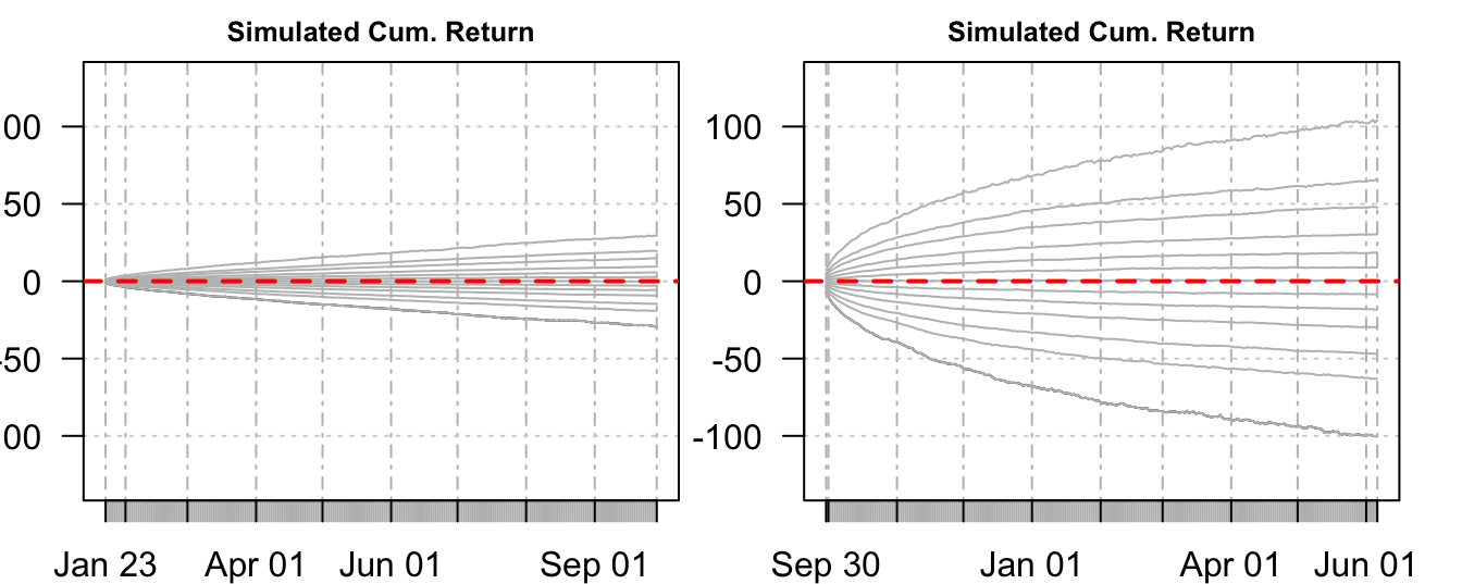
Figure 7.10: Quantiles of the simulated distribution of the cumulative return produced in January 22, 2007 (left) and in September 29, 2008 (right).

MC simulations make also easy to calculate ES. For each horizon \(k\), ES can be calculated as the average of those simulated returns that are smaller than VaR. The code below shows these steps for the two dates considered and Figure 7.11 compare the two risk measures conditional on being on January 22, 2007 and on September 29, 2008. Similarly to the earlier discussion, ES provides a larger (in absolute value) potential loss relative to VaR, a difference that increases with the horizon \(k\).

VaR    = xts(apply(Rcum, 1, quantile, probs=0.01), order.by=futdates)
VaRmat = matrix(VaR, K, S, byrow=FALSE)
Rviol  = Rcum * (Rcum < VaRmat)
ES     = xts(rowSums(Rviol) / rowSums(Rviol!=0), order.by=futdates)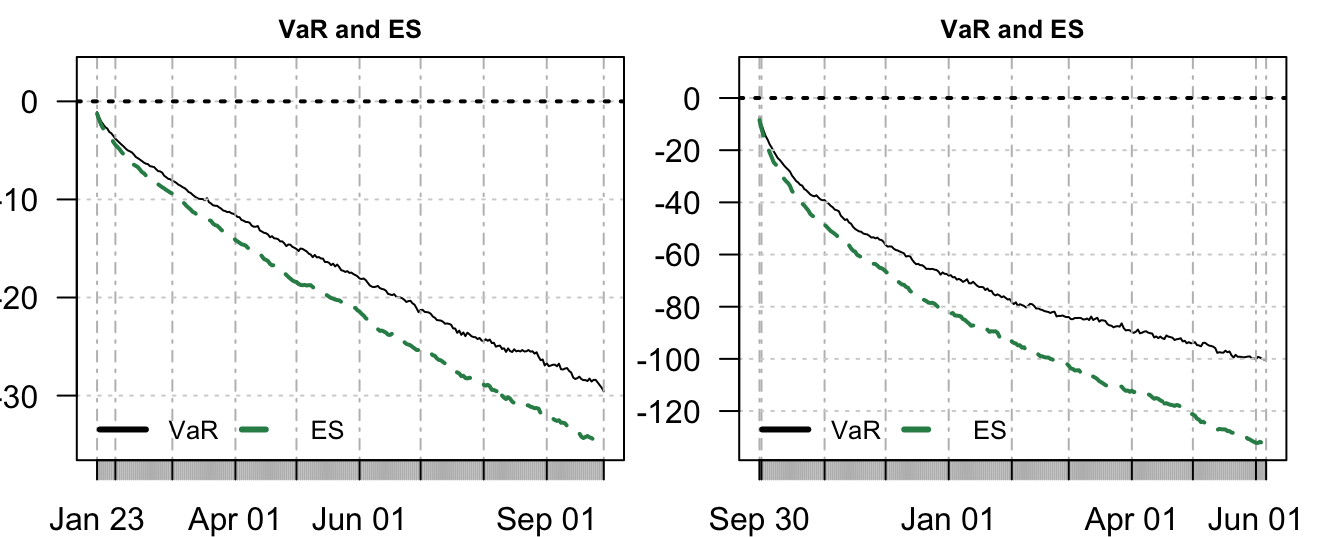

Figure 7.11: VaR and ES for holding periods from 1 to 250 days produced in January 22, 2007 (left) and in September 29, 2008 (right).

7.3.2 Filtered Historical Simulation (FHS)

Filtered Historical Simulation (FHS) combines aspects of the parametric and the HS approaches to risk calculation. This is done by assuming that the volatility of the portfolio return can be modeled with, e.g., EMA or a GARCH specification, while the non-parametric HS approach is used to model the standardized returns \(\epsilon_{t+1} = R_{t+1}/\sigma_{t+1}\). It can be considered a simulation method since the only difference with the MC method discussed above is that the random draws from the standardized returns are used to generate simulated returns instead of draws from a parametric distribution (e.g., normal or \(t\)). This method might be preferred when the risk manager is uncomfortable making assumptions about the shape of the distribution, either in terms of the thickness of the tails or the symmetry of the distribution. In R this method is implemented by replacing the command rnorm(S) that generates a random normal sequence of length \(S\) with sample(std.resid, S, replace=TRUE), where std.resid represents the standardized residuals. This command produces a sample of length S of values randomly taken from the std.resid series. Hence, we are not generating new data, but we are simply taking different samples of the same standardized residuals so that to preserve their distributional properties.

Figure 7.12 compares the MC and FHS approaches in terms of the expected volatility of the daily returns (i.e., average volatility at each horizon \(k\) across the \(S\) simulations) and 99% VaR (i.e., 0.01 quantile of the simulated cumulative returns) for the two forecasting dates that we are considering. The expected future volatility by FHS converges at a slightly lower speed relative to MC during periods of low volatility, while the opposite is true when the forecasting point occurs during a period of high volatility. This is because FHS does not restrict the shape of the distribution on the left tail (as MC does given the assumption of normality) so that large negative standardized returns contribute to determine future returns and volatility. Of course, this result is specific to the S&P 500 daily returns that we are considering as an illustrative portfolio and it might be different when analyzing other portfolio returns.

In terms of VaR calculated on cumulative returns we find that FHS predicts lower risk relative to MC at long horizon, with the difference becoming larger and larger as the horizon \(K\) progresses. Hence, while at short horizons the VaR forecasts are quite similar, they become increasingly different at longer horizon.

# standardized residuals
std.resid  = as.numeric(residuals(fitgarch, standardize=TRUE))
std.resid1 = as.numeric(residuals(fitgarch1, standardize=TRUE))

for (i in 2:K)
{
  Sigma.fhs[i,]  = (gcoef['omega'] + gcoef['alpha1'] * R.fhs[i-1,]^2 + 
                  gcoef['beta1'] * Sigma.fhs[i-1,]^2)^0.5   
  R.fhs[i,]  = sample(std.resid, S, replace=TRUE) * Sigma.fhs[i,]
  Sigma.fhs1[i,]  = (gcoef1['omega'] + gcoef1['alpha1'] * R.fhs1[i-1,]^2 + 
                  gcoef1['beta1'] * Sigma.fhs1[i-1,]^2)^0.5   
  R.fhs1[i,]  = sample(std.resid1, S, replace=TRUE) * Sigma.fhs1[i,]
}

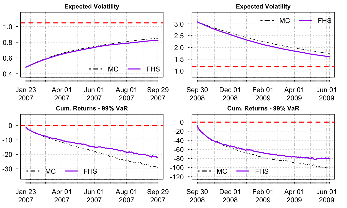
Figure 7.12: Comparison of MC and FHS volatility and 99% VaR produced in January 22, 2007 (left) and in September 29, 2008 (right).

7.4 VaR for portfolios

So far we discussed the simple case of a portfolio composed of only one asset and calculated the Value-at-Risk for such position. However, financial institutions hold complex portfolios that include many assets and expose them to several types of risks. How do we calculate \(VaR\) for such diversified portfolios?

Let’s first characterize the portfolio return as a weighted average of the individual asset returns, that is, \[ R_{t+1}^p = \sum_{j=1}^J w_{j} R_{t+1,j} \] where \(R_t^p\) represents the portfolio return in day \(t\), and \(w_{j}\) and \(R_{j,t}\) are the weight and return of asset \(j\) in day \(t\) (and there is a total of \(J\) assets). To calculate VaR for this portfolio we need to model the distribution of \(R_t^p\). If we assume that the underlying assets are normally distributed, then also the portfolio return is normally distributed and we only need to estimate its mean and standard deviation. In the case of 2 assets (i.e., \(J=2\)) the expected return of the portfolio return is given by \[ E(R_{t+1}^p) = \mu_{t+1,p} = w_{1}\mu_{t+1,1} + w_{2}\mu_{t+1,2} \] which is the weighted average of the expected return of the individual assets. The portfolio variance is equal to \[ Var(R_{t+1}^p) = \sigma^2_{t+1,p} = w_{1}^2\sigma^2_{t+1,1} + w_{2}^2 \sigma^2_{t+1,2} + 2 w_{1} w_{2} \rho_{t+1,12}\sigma_{t+1,1}\sigma_{t+1,2} \] which is a function of the individual (weighted) variances and the correlation between the two assets, \(\rho_{1,2}\). The portfolio Value-at-Risk is then given by \[ \begin{array}{rl} VaR^{0.99}_{t+1,p} =& \mu_{t+1,p} - 2.33 \sigma_{t+1,p}\\ =& w_{1}\mu_{t+1,1} + w_{2}\mu_{t+1,2} - 2.33 \sqrt{w_{1}^2\sigma^2_{t+1,1} + w_{2}^2 \sigma^2_{t+1,2} + 2 w_{1} w_{2} \rho_{t+1,12}\sigma_{t+1,1}\sigma_{t+1,2}}\\ \end{array} \] In case it is reasonable to assume that \(\mu_1 = \mu_2 = 0\), the \(VaR^{0.99}_{t,p}\) formula can be expressed as follows: \[ \begin{array}{rl} VaR^{0.99}_{p,t} = & - 2.33 \sqrt{ w_{1}^2\sigma^2_{t+1,1} + w_{2}^2 \sigma^2_{t+1,2} + 2 w_{1} w_{2} \rho_{t+1,12}\sigma_{t+1,1}\sigma_{t+1,2}}\\ = & - \sqrt{ 2.33^2 w_{1}^2\sigma^2_{t+1,1} + 2.33^2 w_{2}^2 \sigma^2_{t+1,2} + 2 * 2.33^2 w_{1} w_{2} \rho_{t+1,12}\sigma_{t+1,1}\sigma_{t+1,2}}\\ = & - \sqrt{(VaR^{0.99}_{t+1,1})^2 + (VaR^{0.99}_{t+1,2})^2 + 2 * \rho_{t+1,12} VaR^{0.99}_{t+1,1}VaR^{0.99}_{t+1,2}}\\ \end{array} \] which shows that the portfolio VaR in day \(t\) can be expressed in terms of the individual VaRs of the assets and the correlation between the two asset returns. Since the correlation coefficient ranges between \(\pm\) 1, the two extreme cases of correlation implies the following VaR:

• \(\rho_{t+1,12} = 1\): \(VaR^{0.99}_{t+1,p} = -\left(|VaR^{0.99}_{t+1,1}| + |VaR^{0.99}_{t+1,2}|\right)\) the two assets are perfectly correlated and the total portfolio VaR is the sum of the individual VaRs
• \(\rho_{t+1,12} = -1\): \(VaR^{0.99}_{t+1,p} = - |VaR^{0.99}_{t+1,1}-VaR^{0.99}_{t+1,2}|\) the two assets have perfect negative correlation then the total risk of the portfolio is given by the difference between the two VaRs since the risk in one asset is offset by the other asset, and vice versa.

In the Equations above we added a \(t\) subscript also to the correlation coefficient, that is, \(\rho_{t+1,12}\) represents the correlation between the two asset conditional on the information available up to that day. There is evidence supporting the fact that correlations between assets might be changing over time in response to market events or macroeconomic shocks (e.g., a recession). In the following Section we discuss some methods that can be used to model and predict correlations.

7.4.1 Modeling correlations

A simple approach to modeling correlations consists of using MA and EMA smoothing similarly to the case of forecasting volatility. However, in this case the object to be smoothed is not the square return, but the product of the returns of asset 1 and 2 (N.B.: we are implicitly assuming that the mean of both assets can be set equal to zero). Denote the return of asset 1 by \(R_{t,1}\), of asset 2 by \(R_{t,2}\), and by \(\sigma_{t,12}\) the covariance between the two assets in day \(t\). We can estimate \(\sigma_{12,t}\) by a MA of \(M\) days: \[ \sigma_{t+1,12} = \frac{1}{M} \sum_{m=1}^M R_{t-m+1,1}R_{t-m+1,2} \] and the correlation is then obtained by dividing the covariance estimate with the standard deviation of the two assets, that is: \[ \rho_{t+1,12} = \sigma_{t+1,12}/\left( \sigma_{t+1,1}*\sigma_{t+1,2}\right) \] In case the portfolio is composed of \(J\) assets then there are \(J(J-1)/2\) asset pairs for which we need to calculate correlations. An alternative approach is to use EMA smoothing which can be implemented using the recursive formula discussed earlier: \[ \sigma_{t+1,12} = (1-\lambda) \sigma_{t,12} + \lambda R_{t,1}R_{t,2} \] and the correlation is obtained by dividing the covariance by the forecasts of the standard deviations for the two assets.

To illustrate the implementation in R we assume that the firm is holding a portfolio that invests a fraction \(w_1\) in a gold ETF (ticker: GLD) and the remaining fraction \(1-w_1\) in the S&P 500 ETF (ticker: SPY). The closing prices are downloaded from Yahoo Finance starting in Jan 03, 2005 and ending on May 10, 2017 and the goal is to forecast portfolio VaR for the following day. We will assume that the expected daily returns for both assets are equal to zero and forecast volatilities and the correlation between the assets using EMA with \(\lambda=0.06\). In the code below R represents a matrix with 3110 rows and two columns representing the GLD and SPY daily returns.

data     <- getSymbols(c("GLD", "SPY"), from="2005-01-01") 
R        <- 100 * merge(ClCl(GLD), ClCl(SPY))
names(R) <- c("GLD","SPY")
prod     <- R[,1] * R[,2]
cov      <- EMA(prod, ratio=0.06)  # EMA for the product of returns
sigma    <- do.call(merge, lapply(R^2, FUN = function(x) EMA(x, ratio=0.06)))^0.5
names(sigma) <- names(R)
corr     <- cov / (sigma[,1] * sigma[,2])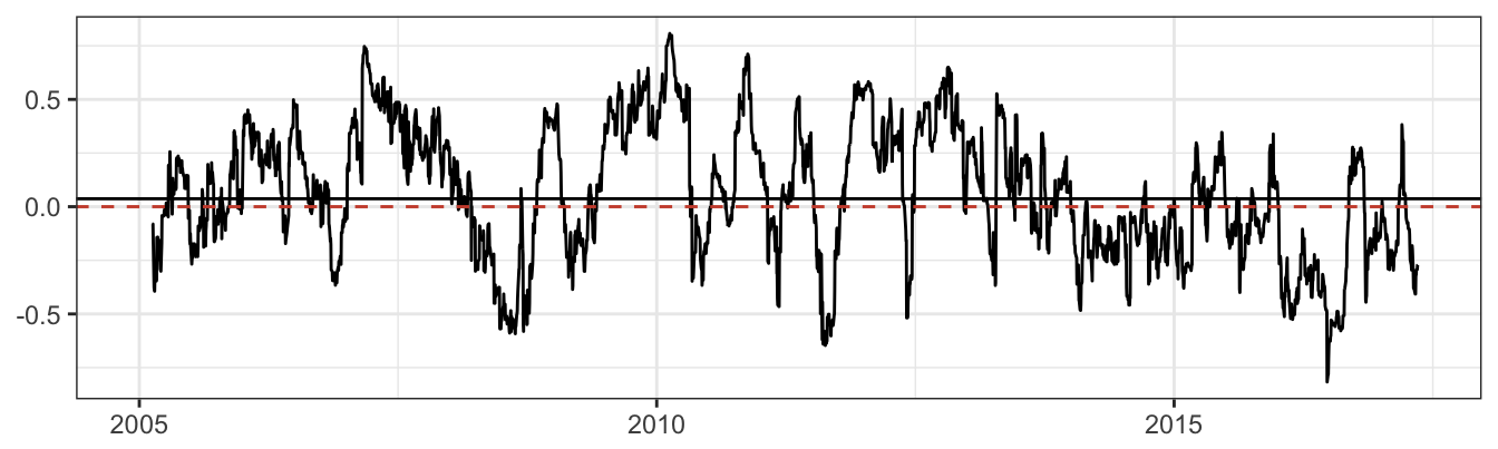

Figure 7.13: Time-varying correlation between GLD and SPY estimated using EMA(0.06).

The time series plot of the EMA correlation in Figure 7.13 shows that the dependence between the gold and S&P 500 returns oscillates significantly around the long-run correlation of NA. In certain periods gold and the S&P 500 have positive correlation as high as 0.81 and in other periods as low as -0.82. During 2008 the correlation between the two assets became large and negative since investors fled the equity market toward gold that was perceived as a safe haven during turbulent times. Based on these forecasts of volatilities and correlation, portfolio VaR can be calculated in R as follows:

w1  = 0.5     # weight of asset 1
w2  = 1 - w1  # weight of asset 2
VaR = -2.33 * ( (w1*sigma[,1])^2 + (w2*sigma[,2])^2 + 
                  2*w1*w2*corr*sigma[,1]*sigma[,2] )^0.5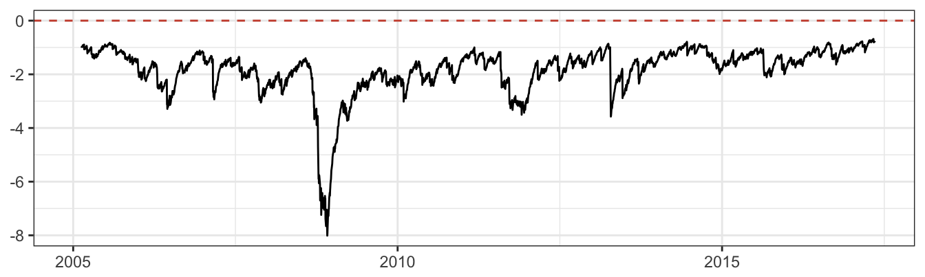

Figure 7.14: 99% VaR for a portfolio of GLD and SPY.

The one-day portfolio Value-at-Risk fluctuates substantially between -0.68% and -8.01%, which occurred during the 2008-09 financial crises. It is also interesting to compare the portfolio VaR with the risk measure if the portfolio is fully invested in either asset. The time series graph below shows the VaR for three scenarios: a portfolio invested 50% in gold and equity, 100% gold, and 100% S&P 500. Portfolio VaR is between the VaRs for the individual assets when correlation is positive. However, in those periods in which the two assets have negative correlation (e.g., 2008) the portfolio VaR is higher than both individual VaRs since the two assets are moving in opposite directions and the risk exposures partly offset each other.

VaRGLD = -2.33 * sigma[,1]
VaRSPY = -2.33 * sigma[,2]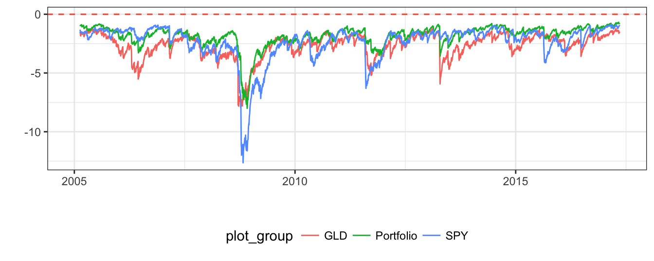

Figure 7.15: Comparison of 99% VaR for a portfolio invested in GLD and SPY, and for a position that is fully invested in GLD or SPY.

7.5 Backtesting VaR

In the risk management literature backtesting refers to the evaluation/testing of the properties of a risk model based on past data. The approach consists of using the risk model to calculate VaR based on the information (e.g., past returns) that was available to the risk manager at that point in time. The VaR forecasts are then compared with the actual realization of the portfolio return to evaluate if they satisfy the properties that we expect should hold for a good risk model. One such characteristic is that the coverage of the risk model, defined as the percentage of returns smaller than VaR, should be close to 100*(1-\(\alpha\))%. In other words, if we are testing VaR with \(\alpha\) equal to 0.01 we should expect, approximately, 1% of days with violations. If we find that returns were smaller than \(VaR\) significantly more/less often than 1%, then we conclude that the model has inappropriate coverage. For the S&P 500 return and VaR calculated using the EMA method the coverage is equal to

V = na.omit(lag(sp500daily,1) <= var)
T1  = sum(V)
TT   = length(V)
alphahat = mean(T1/TT)

[1] 0.011

In this case, we find that the 99% VaR is violated as often (0.011) then expected (0.01). We can test the hypothesis that \(\alpha = 0.01\) (or 1%) by comparing the likelihood that the sample has been generated by \(\alpha\) as opposed to its estimate \(\hat{\alpha}\), which in this example is equal to 0.011. One way to test this hypothesis is to define the event of a violation of VaR, that is \(R_{t+1} \leq VaR_{t+1}\), as a binomial random variable with probability \(\alpha\) that the event occurs. Since we have a total of \(T\) days and introducing the assumption that violations are independent of each other, then the joint probability of having \(T_1\) violations (out of \(T\) days) is \[ \mathcal{L}(\alpha, T_1, T) = \alpha^{T_1} (1-\alpha)^T_0 \] where \(T_0 =T - T_1\). The hypothesis \(\alpha = 0.01\) can be tested by comparing this likelihood above at the estimated \(\alpha\) and at the theoretical value of 0.01 (more generally, if VaR is calculated at 95% then \(\alpha\) is 0.05). This type of tests are called likelihood ratio tests and can be interpreted as the distance between the theoretical value (i.e., using \(\alpha = 0.01\)) of the likelihood of obtaining \(T_1\) violation in \(T\) days and the likelihood based on the sample estimate \(\hat{\alpha}\). The statistic and distribution of the test for Unconditional Coverage (UC) are \[ {UC}=-2\ln\left(\frac{\mathcal{L}(0.01,T_1, T)}{\mathcal{L}(\hat\alpha,T_1, T)}\right) \sim \chi^2_1 \] where \(\hat\alpha = T_1/T\) and \(\chi^2_1\) denotes the chi-square distribution with 1 degree-of-freedom. The critical values at 1, 5, and 10% are 6.63, 3.84, and 2.71, respectively, and the null hypothesis \(\alpha = 0.01\) is rejected if \(LR^{UC}\) is larger than the critical value. In practice, the test statistic can be calculated as follows: \[ -2 \left[ T_1 \ln\left(\frac{0.01}{\hat\alpha}\right) + T_0 \ln\left(\frac{0.99}{1-\hat\alpha}\right)\right] \] In the example discussed above we have \(\hat\alpha =\) 0.011, \(T_1=\) 74, and \(T\) is 6862. The test statistic is thus

UC  = -2 * ( T1 * (log(0.01/alphahat)) 
             + (TT - T1) * log(0.99/(1-alphahat))) 

Since 0.386 is smaller than 3.84 we do not reject the null hypothesis at 5% significance level that \(\alpha = 0.01\) and conclude that the risk model provides appropriate coverage.

While testing for coverage, we introduced the assumption that violations are independent of each other. If this assumption fails to hold, then a violation in day \(t\) has the effect of increasing/decreasing the probability of experiencing a violation in day \(t+1\), relative to its unconditional level. A situation in which this might happen is during financial crises when markets enter a downward spiral which is likely to lead to several consecutive days of violations and thus to the possibility of underestimating risk. The empirical evaluation of this assumption requires the calculation of two probabilities: 1) the probability of having a violation in day \(t\) given that a violation occurred in day \(t-1\), and 2) the probability of having a violation in day \(t\) given that no violation occurred the previous day. We denote the estimates of these conditional probabilities as \(\hat\alpha_{1,1}\) and \(\hat\alpha_{0,1}\), respectively. They can be estimated from the data by calculating \(T_{1,1}\) and \(T_{0,1}\) that represent the number of days in which a violation was preceded by a violation and a no violation, respectively. In R we can determine these quantities as follows:

T11 = sum((lag(V,1)==1) & (V==1))
T01 = sum((lag(V,1)==0) & (V==1))

where we obtain that \(T_{0,1} =\) 74 and \(T_{1,1} =\) 0, with their sum equal to \(T_1\). Similarly, we can calculate \(T_{1,0}\) and \(T_{0,0}\) and the estimates are NA and NA, respectively, that sum to \(T_0\). Since we look at violations in two consecutive days we lose one observation and our total sample size is now \(T-1 =\) 400. We can then calculate the conditional probabilities of a violation in a day given that the previous day there was no violation as \(\hat\alpha_{0,1} = T_{0,1} / (T_{0,1}+T_{1,1})\) while the probability of a violation in two consecutive days, that is, \(\hat\alpha_{1,1} = 1-\hat\alpha_{0,1} = T_{1,1} / (T_{0,1}+T_{1,1})\). Similarly, we can calculate \(\hat\alpha_{1,0}\) and \(\hat\alpha_{0,0}\). For the daily S&P 500 introduced earlier, the estimates are \(\hat\alpha_{1,1}=\) 0 and \(\hat\alpha_{0,1}=\) 1, and \(\hat\alpha_{1,0}=\) NA and \(\hat\alpha_{0,0}=\) NA. While we have an overall estimated probability of a violation of 1.1%, this probability is equal to 0% after a day in which the risk model was violated and NA% following a day without a violation. Since these probabilities are significantly different from each other, we should conclude that the violations are not independent over time. To make this conclusion in statistical terms, we can statistically test the hypothesis of independence of the violations by stating the null hypothesis as \(\alpha_{0,1} = \alpha_{1,1} = \alpha\) which can be tested using the same likelihood ratio approach discussed earlier. In this case, the statistic is calculated as the ratio of the likelihood under independence, \(\mathcal{L}(\hat\alpha,T_1,T)\), relative to the likelihood under dependence, which we denote by \(\mathcal{L}(\hat\alpha_{0,1},\hat\alpha_{1,1},T_{0,1},T_{1,1},T)\) which is given by \[ \mathcal{L}(\hat\alpha_{0,1},\hat\alpha_{1,1},T_{0,1},T_{1,1},T) = \hat\alpha_{1,0}^{T_{1,0}} (1-\hat\alpha_{1,0})^{T_{1,1}} \hat\alpha_{0,1}^{T_{0,1}} (1-\hat\alpha_{0,1})^{T_{0,0}} \] the test statistic and distribution for the hypothesis of Independence (IND) in this case is \[ IND = -2\ln\left(\frac{\mathcal{L}(\hat\alpha,T_{0},T)}{\mathcal{L}(\hat\alpha_{0,1},\hat\alpha_{1,1},T_{0,1},T_{1,1},T)} \right) \sim \chi^2_1 \]

and the critical values are the same as for the UC test. The numerator of the IND test is the likelihood in the denominator of the UC test and it is based on the empirical estimate of \(\alpha\) rather than the theoretical value \(\alpha\). The value of the \(IND\) test statistic is NA which is smaller relative to the critical value at 5% so that we do not reject the null hypothesis that the violations occur independently.

Finally, we might be interested in testing the hypothesis \(\alpha_{0,1} = \alpha_{1,1} = 0.01\) which tests jointly the independence of the violations as well as the coverage which should be equal to 1%. This test is referred to as Conditional Coverage and the test statistic is given by the sum of the previous two test statistics, that is, \(CC = IND + UC\) and it is distributed as a \(\chi^2_2\). The critical values at 1, 5, and 10% in this case are 9.21, 5.99, and 4.61, respectively.

R commands

Exercises

1. Exercise 1
2. Exercise 2

Adrian, Tobias, Richard K Crump, and Erik Vogt. 2015. “Nonlinearity and Flight to Safety in the Risk-Return Trade-Off for Stocks and Bonds.” Federal Reserve of New York Working Paper.

Albert, Jim, and Maria Rizzo. 2012. R by Example. Springer Science & Business Media.

Engle, Robert F. 1982. “Autoregressive Conditional Heteroscedasticity with Estimates of the Variance of United Kingdom Inflation.” Econometrica, 987–1007.

Fama, Eugene F, and Kenneth R French. 1993. “Common Risk Factors in the Returns on Stocks and Bonds.” Journal of Financial Economics 33 (1). Elsevier: 3–56.

Newey, Whitney K., and Kenneth D. West. 1987. “A Simple, Positive Semi-Definite, Heteroskedasticity and Autocorrelation Consistent Covariance Matrix.” Econometrica 55: 703–8.

Shiller, Robert J. 2015. Irrational Exuberance. Princeton University Press.

Stock, James H, and Mark W Watson. 2010. Introduction to Econometrics. Addison Wesley.

Tsay, Ruey S. 2005. Analysis of Financial Time Series. Vol. 543. John Wiley & Sons.

Welch, Ivo, and Amit Goyal. 2008. “A Comprehensive Look at the Empirical Performance of Equity Premium Prediction.” Review of Financial Studies 21 (4). Soc Financial Studies: 1455–1508.

Wickham, Hadley. 2009. Ggplot2: Elegant Graphics for Data Analysis. Springer Science & Business Media.

Wooldridge, Jeffrey M. 2015. Introductory Econometrics: A Modern Approach.

Zuur, Alain, Elena N Ieno, and Erik Meesters. 2009. A Beginner’s Guide to R. Springer Science & Business Media.